In this article I wrote about financial stock performance across the typical four-year election cycle. To make a long story short, using ticker FSRBX as a proxy for the sector there appear to be four “favorable” periods within the election cycle.
The last of those four begins on July 1st and ends
December 31st.
Please DO NOT confuse that statement with me shouting “BUY FINANCIAL
STOCKS NOW!” In fact, I am not “predicting”
anything. As always, one can come up
with plenty of good reasons NOT to do that right now. Nothing – especially when it comes to
seasonality in the stock market – is ever “guaranteed”. But just a quick review.
A Quick Review
Figure 1 displays the total return for FSRBX ONLY during the
months of July through December of each presidential election year since fund inception
in 1986.
Figure 1 – Cumulative Return for FSRBX during July through December
of Election Years; 1986-2020
Figure 2 displays the cumulative return on an election year by
election year basis.
Figure 2 – FSRBX during Jul-Dec of Election Years; 1986-2020
Summary
There is plenty of negative sentiment out there regarding
financial stocks. But historically the
months directly ahead have been favorable for this sector. Investors willing to buck the crowd might
consider giving financial stocks the benefit of the doubt in the months ahead.
See also Jay Kaeppel Interview in July 2020 issue of Technical Analysis of Stocks and Commodities magazine
Disclaimer: The information, opinions and ideas expressed herein are for
informational and educational purposes only and are based on research conducted
and presented solely by the author. The
information presented represents the views of the author only and does not
constitute a complete description of any investment service. In addition, nothing presented herein should
be construed as investment advice, as an advertisement or offering of
investment advisory services, or as an offer to sell or a solicitation to buy
any security. The data presented herein
were obtained from various third-party sources.
While the data is believed to be reliable, no representation is made as
to, and no responsibility, warranty or liability is accepted for the accuracy
or completeness of such information.
International investments are subject to additional risks such as
currency fluctuations, political instability and the potential for illiquid
markets. Past performance is no
guarantee of future results. There is
risk of loss in all trading. Back tested
performance does not represent actual performance and should not be interpreted
as an indication of such performance.
Also, back tested performance results have certain inherent limitations
and differs from actual performance because it is achieved with the benefit of
hindsight.
This post stems entirely from a tweet from Mark Ungewitter. Mark is a Senior Vice President & Investment Officer at Charter Trust Company and has a very interesting twitter feed.
He recently posted the shot you see in Figure 1.
Figure 1 – Mark Ungewitter tweet regarding S&P 500 4-week
and 40-week averages (Courtesy: www.Twitter.com)
The calculation is pretty straightforward:
A = 4-week average of S&P 500 closes
B = 40-week average of S&P 500 closes
C = A / B
What I will heretofore refer to as an “MU Buy Signal” occurs
when the following two steps are completed:
*The ratio (Value C above) falls to 0.95 or below
*The ratio (Value C above) subsequently rises to 1.03 or above
In slightly clearer terms, when the 4-week average drops 5% or
more below the 40-week average it indicates an oversold market and sets the
stage for the next bull market. The new
bull market is confirmed (at least in most cases) when the 4-week average subsequently
rises 3% or more above the 40-week average.
Results
Is there any real value in this calculation? You be the judge. Let’s consider the average 4, 13, 26, 39 and
52 week returns following such buy signals versus the average return for all 4,
13, 26, 39- and 52-week periods.
To understand, the right-hand column in row two of Figure 2 tells
us the historical average 4-week return for the S&P 500 Index is +0.5%. However, as you can see in the second column
in row two, the average 4-week return following MU Buy Signals is +2.3%.
The key thing to note is that across all time frames the average S&P 500 return after a MU buy signal are significantly higher than the typical return for that period.
Figure 2 – S&P 500 returns after MU Buy Signals versus all weeks
Consistency – more specifically defined as “probability of
profit” – is also important. Figure 3
displays the typical percent of time the S&P 500 moves higher over 4, 13,
26, 39 and 52-week period in the far-right hand column.
Note again that for each time period the “% of times UP” is significantly higher following a MU Buy signal.
Figure 3 – % time S&P 500 higher x-weeks after MU Buy Signals
To illustrate one last highlight of consistency, Figure 4
displays the cumulative % price return for the S&P 500 Index if held ONLY
during the 39-weeks after each MU Buy Signal since 1932.
Figure 4 – Cumulative % +(-) if S&P 500 Index is held for 39-weeks after each MU Buy Signal
For the record, since 1958 17 of the last 18 MU Buy Signals have seen the S&P 500 Index rise in the 39-weeks following the signal.
Summary
Looks like something worth following to me. Thanks Mark.
See also Jay Kaeppel Interview in July 2020 issue of Technical Analysis of Stocks and Commodities magazine
Figure 5 below displays the S&P performance following previous MU Buy Signals. IMPORTANT DISCLAIMER: The data in Figure 5 is generated using my own set of price data which is believed to be accurate. It is possible Mark Ungewitter could generate slightly different results.
Figure 5 – MU Buy Signals (as generated by Jay’s database) and S&P 500 Performance
Jay
Kaeppel
Disclaimer: The information, opinions and ideas expressed herein are for
informational and educational purposes only and are based on research conducted
and presented solely by the author. The
information presented represents the views of the author only and does not constitute
a complete description of any investment service. In addition, nothing presented herein should
be construed as investment advice, as an advertisement or offering of
investment advisory services, or as an offer to sell or a solicitation to buy
any security. The data presented herein
were obtained from various third-party sources.
While the data is believed to be reliable, no representation is made as
to, and no responsibility, warranty or liability is accepted for the accuracy
or completeness of such information.
International investments are subject to additional risks such as
currency fluctuations, political instability and the potential for illiquid
markets. Past performance is no
guarantee of future results. There is
risk of loss in all trading. Back tested
performance does not represent actual performance and should not be interpreted
as an indication of such performance.
Also, back tested performance results have certain inherent limitations
and differs from actual performance because it is achieved with the benefit of
hindsight.
In case you were not aware, I am something of a seasonality “junkie”. Hey, if you gotta have a vice…
Anyway, as it turns out many individual months have a “personality”
of their own. Take July for
instance.
July, Interrupted
We will break July into two parts:
*Part 1 includes:
-Trading days #1 through 13 (i.e., the first 13 trading days of the month, i.e., excludes holidays and weekends and includes only actual trading days when the market is open) AND
-Trading days #17 through #21.
*Part 2 includes:
-ALL other trading days of July (i.e., trading days #14 through 16 and anything after trading day #21)
Figure 1 displays the cumulative growth for the Dow Jones Industrial
Average during all Part 1 days ONLY starting in 1936.
Figure 1 – Cumulative Dow price % +(-) during July Favorable Days (1936-2019)
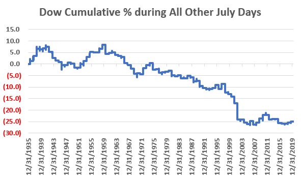
Figure 2 displays the cumulative growth for the Dow Jones Industrial
Average during all Part 2 days ONLY starting in 1936.
Figure 2 – Cumulative Dow price % +(-) during July Non-Favorable Days (1936-2019)
In a nutshell:
Figure 3 – Summary of Performance for July Favorable versus Non-Favorable Trading Days (1936-2019)
For 2020, the first favorable period includes July 1 through July 20 and the 2nd includes July 24 through July 30.
Is it worth it to trade in and out during the month of July? That’s up to you to decide. But for what it’s worth, here are the numbers.
See also Jay Kaeppel Interview in July 2020 issue of Technical Analysis of Stocks and Commodities magazine
Disclaimer: The information, opinions and ideas expressed herein are for
informational and educational purposes only and are based on research conducted
and presented solely by the author. The
information presented represents the views of the author only and does not
constitute a complete description of any investment service. In addition, nothing presented herein should
be construed as investment advice, as an advertisement or offering of
investment advisory services, or as an offer to sell or a solicitation to buy
any security. The data presented herein
were obtained from various third-party sources.
While the data is believed to be reliable, no representation is made as
to, and no responsibility, warranty or liability is accepted for the accuracy
or completeness of such information.
International investments are subject to additional risks such as
currency fluctuations, political instability and the potential for illiquid
markets. Past performance is no
guarantee of future results. There is
risk of loss in all trading. Back tested
performance does not represent actual performance and should not be interpreted
as an indication of such performance.
Also, back tested performance results have certain inherent limitations
and differs from actual performance because it is achieved with the benefit of
hindsight.
That number is 25,383.11. The Dow needs to close above this level on June 30th. If it does, that will complete a “2nd Quarter Trifecta”, i.e., a 2nd quarter of the year during which April, May and June all show a monthly gain.
Why might this matter?
Let’s consider a little history.
The History of the 2nd Quarter Trifecta
For our purposes, we will consider the 9 months (July through the following March) following a 2nd Quarter Trifecta to be “favorable” for stocks. So, for our test each time the Dow shows a gain for April AND May AND June in the same year we will buy and hold the Dow for 9 months. During all other months no gain or loss is accrued.
Figure 1 shows the cumulative gain for this “strategy” starting
back in 1901.
Figure 1 – Dow cumulative % +(-) during 9 months following
The key thing to note about Figure 1 is that the equity curve
exhibits what I like to call “LLUR” – which stands for “Lower Left to Upper
Right”, which is how we like our equity curves to look.
Figure 2 shows the actual results on a case-by-case basis.
Figure 2 – Dow price performance in 9 months after 2nd Quarter Trifecta
Figure 3 displays a summary of these occurrences.
Figure 3 – Dow performance summary for 9-months after 2nd Quarter Trifecta signals
Things to note:
*Following a 2nd Quarter Trifecta signal, the Dow has
not registered a 9-month loss since 1919-1920, a string of 13 consecutive
winning trades
*The average 9-month gain was +15% versus an average loss of -1%
*The worst 9-month loss was just -3% following the 1919 signal
Summary
So, you can see why 25,383.11 is an important price level for
the Dow. If it closes June above that
level does that guarantee that the Dow will be higher by the end of March
2021? Not at all. But it does add another significantly
favorable piece of history to the weight of the evidence.
See also Jay Kaeppel Interview in July 2020 issue of Technical Analysis of Stocks and Commodities magazine
Disclaimer: The information, opinions and ideas expressed herein are for
informational and educational purposes only and are based on research conducted
and presented solely by the author. The
information presented represents the views of the author only and does not
constitute a complete description of any investment service. In addition, nothing presented herein should
be construed as investment advice, as an advertisement or offering of
investment advisory services, or as an offer to sell or a solicitation to buy
any security. The data presented herein
were obtained from various third-party sources.
While the data is believed to be reliable, no representation is made as
to, and no responsibility, warranty or liability is accepted for the accuracy
or completeness of such information.
International investments are subject to additional risks such as
currency fluctuations, political instability and the potential for illiquid
markets. Past performance is no
guarantee of future results. There is
risk of loss in all trading. Back tested
performance does not represent actual performance and should not be interpreted
as an indication of such performance.
Also, back tested performance results have certain inherent limitations
and differs from actual performance because it is achieved with the benefit of
hindsight.
I am fond of saying that the primary key to investment and trading success is finding an “edge” and exploiting it repeatedly. I don’t know, sounds reasonable. But what constitutes an “edge”? Well, one definition that comes to mind is “some tidbit of information that leads to consistent profits”. So, what I will highlight here is simply that – a tidbit of information. It is probably not enough to go on as a standalone approach. And it comes around very infrequently (only 5 times every four years), and won’t come up again until 2021. So, chances are you will forget all about this by then. But hey, that’s not my problem, I’m just the “idea guy.”
See also Jay Kaeppel Interview in July 2020 issue of Technical Analysis of Stocks and Commodities magazine
The Big 5 Months
For the record, The Big 5 Months came about from a lot of work that I have done analyzing the four-year election cycle. For the sake of brevity, I’ll not be getting into the “how this came about” part, just the “here’s what it is” part.
The Big 5 Months is comprised of the following months within the four-year election cycle.
*April of the Post-Election Year
*December of the Post-Election Year
*November of the Mid-Term Election Year
*April of the Pre-Election Year
*December of the Pre-Election Year
To help visualize this calendar, see Figure 1.
Figure 1 – The Big 5 Months Calendar
Unfortunately, there are no months within the actual Presidential Election year that qualify. Why do these months matter? First note that results are measured from January 1901 through May 2020 using month-end price data for the Dow Jones Industrial Average. December of 2020 will mark the end of the 30th election cycle during that time period. Through May of 2020 this comes to a total of 1432 months. The Big 5 Months comprise only 150 total months, or 10.5% of all months.
So again, what’s the big deal amount these months? In my best Maxwell Smart voice let me say “Would you believe?” then I would ask you to consider the results displayed in Figure 2.
Figure 2 – Results: Big 5 Months versus All Other Months; 1901-May 2020
To put this into context consider that:
*Although The Big 5 Months comprised only 10.5% of all months in
the past 119+ years of trading, within those months the Dow registered 10.9
times as much gain as during the other 89.5% of months.
Figure 3 displays the cumulative % price performance for the Dow
during “The Big 5” months versus “All Other Months.”
Figure 3 – Cumulative price performance %: The Big 5 Months versus All Other Months; 1901-May 2020
Drilling Down
Taken individually the results for each of The Big 5 Months is decent but not exactly jaw-dropping. See Figure 4.
Figure 4 – The Big 5 performance by Month; 1901-May 2020
When taken collectively however, the results are fairly impressive:
*Holding the Dow only during The Big 5 Months every four years registered a gain during 28 of the 30 election cycles, or 93% of the time
*Holding the Dow only during All Other Months every four years (through
May 2020) registered a gain during 19 of the 30 election cycles, or 63% of the
time
*Holding the Dow only during The Big 5 Months every four years outperformed holding the Dow during the other 43 months every four years 18 out of 30 times**
**there are still seven months to complete during 30th election cycle ending December 2020. But so far, from January 2017 through May 2020, The Big 5 Months have gained +21.7% versus +5.6% for All Other Months.
Summary
Opportunity is where you find it. Do The Big 5 Months constitute an opportunity? That’s not for me to say. Will anyone remember this come April of 2021? Will April of 2021 even see the Dow register a gain?
Dunno. But remember, opportunity is where you find it.
See also Jay Kaeppel Interviewin
July 2020 issue of Technical Analysis of Stocks and Commodities magazine
Disclaimer: The information, opinions and ideas expressed herein are for
informational and educational purposes only and are based on research conducted
and presented solely by the author. The
information presented represents the views of the author only and does not constitute
a complete description of any investment service. In addition, nothing presented herein should
be construed as investment advice, as an advertisement or offering of
investment advisory services, or as an offer to sell or a solicitation to buy
any security. The data presented herein
were obtained from various third-party sources.
While the data is believed to be reliable, no representation is made as
to, and no responsibility, warranty or liability is accepted for the accuracy
or completeness of such information.
International investments are subject to additional risks such as
currency fluctuations, political instability and the potential for illiquid
markets. Past performance is no
guarantee of future results. There is
risk of loss in all trading. Back tested
performance does not represent actual performance and should not be interpreted
as an indication of such performance.
Also, back tested performance results have certain inherent limitations
and differs from actual performance because it is achieved with the benefit of
hindsight.
The information contained in this piece is not presented as a “strategy” but rather as an “idea.” Essentially a starting point if you will, for developing a method to exploit certain seasonal trends that the stock market has exhibited over a number of years.
See also Jay Kaeppel Interview in July 2020 issue of Technical Analysis of Stocks and Commodities magazine
The Indexes
*S&P 500 Index (large-cap)
*MSCI EAFE Index (International)
*S&P 400 Index (mid-cap)
*Nasdaq 100** (OTC stocks)
*FTSE NAREIT All Equity Index (Real Estate Investment Trusts)
**I have monthly total return data for the Nasdaq 100 (ticker
NDX) starting in April 1996; so, prior to that date the Nasdaq Composite
(ticker COMPQ) is used
Test Period
January 1981 through May 2020.
The start date of Jan 1981 was chosen because that is the first month of
data available for the S&P 400 Index, so in order to compare apples-to-apples
testing on all indexes are started then.
The Seasonal Periods
Each index has exhibited its own somewhat unique seasonal tendencies over the years. So, it is correct to point out that the seasonal periods used for each index is chosen with the benefit of hindsight and that, yes, “past performance does not guarantee future results.” With that caveat in mind, the periods that each index is held appears in Figure 1
Figure 1 – Favorable Seasonal Periods by Index
Results
Figure 2 – Index % total return during Favorable versus
Unfavorable periods
Figure 3 displays the cumulative total return for each index
ONLY during the Favorable Seasonal Periods highlighted in Figure 1.
Figure 3 – Favorable Periods cumulative % return
Figure 4 displays the cumulative total return for each index
ONLY during the Unfavorable Seasonal Periods – i.e., all months of the year NOT
listed for a given index in Figure 1.
Figure 4 – Unfavorable Periods cumulative % return
The Key Things to Note:
*The difference in overall returns between “Favorable” and “Unfavorable”
periods is stark
*There is no guarantee that any given Favorable period will show
a gain, nor that it won’t show a significant loss
*In most cases it is not necessarily accurate to refer to the “Unfavorable”
period as “Bearish”, since 4 of the 5 indexes show a net gain during the
Unfavorable periods.
Summary
The idea of being fully bullish during a Favorable period and
fully bearish during the Unfavorable period does not guarantee “smooth sailing.”
Still, the bottom line is that seasonality clearly appears to
offer investors an “edge.”
Pushing one’s advantage during the Favorable periods and “picking
one’s spots” during the Unfavorable periods does appear to be a good overarching
theme for investors looking to “beat the market.”
See also Jay Kaeppel Interview in July 2020 issue of Technical Analysis of Stocks and Commodities magazine
Disclaimer: The information, opinions and ideas expressed herein are for
informational and educational purposes only and are based on research conducted
and presented solely by the author. The
information presented represents the views of the author only and does not
constitute a complete description of any investment service. In addition, nothing presented herein should
be construed as investment advice, as an advertisement or offering of
investment advisory services, or as an offer to sell or a solicitation to buy
any security. The data presented herein
were obtained from various third-party sources.
While the data is believed to be reliable, no representation is made as
to, and no responsibility, warranty or liability is accepted for the accuracy
or completeness of such information.
International investments are subject to additional risks such as
currency fluctuations, political instability and the potential for illiquid
markets. Past performance is no
guarantee of future results. There is
risk of loss in all trading. Back tested
performance does not represent actual performance and should not be interpreted
as an indication of such performance.
Also, back tested performance results have certain inherent limitations
and differs from actual performance because it is achieved with the benefit of
hindsight.
It is little recognized that real estate stocks tend to register
the bulk of their gains during the months of March through July plus the month
of December (although March of 2020 was obviously a very “unpretty” exception). Figure 1 displays the cumulative total return
for Fidelity Select Real Estate (ticker FRESX) only during these favored months
since inception in 1986.
Figure 1 – FRESX total return March-July (1986-2020)
(See also Jay Kaeppel Interview in July 2020 issue of Technical Analysis of Stocks and Commodities magazine)
The August-November period has been much less consistent. Figure 2 displays the return for FRESX only
during these months since inception.
Figure 2 – FRESX total return August-November (1986-2020)
So hopefully the rest of June plus the month of July will be
favorable for REITs (Real Estate Investment Trusts) in general and will recoup
more of the March 2020 loss.
Drilling a Little Deeper
Just for fun, lets “get into the (seasonal) weeds” for real
estate. Again, using FRESX as a proxy
(although we will have to use another vehicle for trading purposes – more in a
moment), the period below has seen some fairly consistent gains. That period consists of:
*26 trading days
*Following June Trading Day of the Month #17
(did I mention we were getting into the weeds?)
The next period starts at the close on 6/23/2020 (which is the
17th trading day of June) and extends for 26 trading days through
the end of trading on 7/30/2020.
Will this period show a gain?
Maybe, maybe not. But consider
the history. Figure 3 displays the
cumulative growth achieved by holding FRESX for these same 26 days each year (IMPORTANT
NOTE: If you actually did this with FRESX Fidelity would likely charge a
switching fee for NOT holding it for 29 days – so we will discuss an
alternative momentarily).
Figure 3 – FRESX cumulative % +(-) during 26 favorable June/July
trading days
Figure 4 shows results on a year-by-year basis.
Figure 4 – FRESX yearly % +(-) during 26 favorable June/July
trading days
For the record:
*# of times UP = 27 (82% of the time)
*# of times DOWN = 6 (18% of the time)
*Average UP % = +4.0%
*Average DOWN % = (-3.3%)
*Largest UP% = +16.4% (in 2009)
*Largest DOWN % = -6.3% (in 2007)
An Alternative
As I have mentioned, Fidelity charges a (not insignificant) “switching fee” for sector fund trades held less than 29 days – ostensibly to discourage frequent switching. An alternative is the ETF ticker IYR (iShares U.S. Real Estate ETF), which can be bought and sold like shares of stock. IYR has a shorter track record as it started trading in 2000.
ETF ticker IYR history during 26-day favorable June/July Period:
*# of times UP = 17 (85% of the time)
*# of times DOWN = 3 (15% of the time)
*Average UP % = +4.3%
*Average DOWN % = (-4.2%)
*Largest UP% = +16.1% (in 2009)
*Largest DOWN % = -6.3% (in 2007)
As you can see, results using IYR are close enough to those of
FRESX (at least in my market-addled mind) that IYR constitutes a viable trading
alternative.
Summary
Does any of this mean that I am “recommending” that anyone buy IYR
on the close of 6/23/2020, or even that IYR is likely to show a gain in the
subsequent 26 trading days? Sorry folks,
I don’t offer investment advice on this blog.
Everything I write about here is strictly “informational” based on my
own (granted, somewhat unorthodox) way of looking at things.
See also Jay Kaeppel Interview in July 2020 issue of Technical Analysis of Stocks and Commodities magazine
Disclaimer: The information, opinions and ideas expressed herein are for
informational and educational purposes only and are based on research conducted
and presented solely by the author. The
information presented represents the views of the author only and does not
constitute a complete description of any investment service. In addition, nothing presented herein should
be construed as investment advice, as an advertisement or offering of
investment advisory services, or as an offer to sell or a solicitation to buy
any security. The data presented herein
were obtained from various third-party sources.
While the data is believed to be reliable, no representation is made as
to, and no responsibility, warranty or liability is accepted for the accuracy
or completeness of such information.
International investments are subject to additional risks such as
currency fluctuations, political instability and the potential for illiquid
markets. Past performance is no
guarantee of future results. There is
risk of loss in all trading. Back tested
performance does not represent actual performance and should not be interpreted
as an indication of such performance.
Also, back tested performance results have certain inherent limitations
and differs from actual performance because it is achieved with the benefit of
hindsight.
I am pretty sure I write this same article every year – but who can blame me? Soybeans are about to enter one of their most “unfavorable” seasonal periods of the year.
The Seasonal Pattern
Soybeans tend to exhibit weakness between the close of the 14th
trading day of June through the close on the 18th trading day of
July. This year those dates are:
*The close on June 18th through
*The close on July 27th
The History of our Seasonally Unfavorable Period
Figure 1 displays the hypothetical $ +(-) achieved by holding a long 1-lot position in soybean futures from June Trading Day 14 through July Trading Day 18 every year since 1984.
Figure 1 – $ +(-) holding long 1 soybean futures contract June
TDM 14 through July TDM 18
Not a pretty picture.
In sum, this period on a year-to-year basis:
*# of times UP = 10 (28% of the time)
*# of times DOWN = 26 (72% of the time)
*Average gain = +$2,418
*Average loss = (-$5,213)
Figure 2 displays year-by-year results.
Figure 2 – Soybeans year-by-year during “unfavorable” June/July
period
Things to Note
OK, so just because I have written all of this down does that
mean that beans are “guaranteed” to decline between the dates listed
above? Of course not. For the “counter argument” see Figure 3. The top clip shows the daily chart for ticker
SOYB (an ETF that tracks soybean futures) and the bottom clip shows the weekly
chart for SOYB.
Figure 3 – Daily and Weekly charts for ticker SOYB with Elliott Wave Counts (Courtesy ProfitSource by HUBB)
Note that BOTH daily and weekly charts have recently completed a 5-wave Elliott Wave decline (according to the algorithm built into ProfitSource software – which I use to generate Elliott Wave counts as I have never been too good at doing it subjectively myself), which suggests that “the bottom may well be in” for soybeans.
So – in theory anyway – we have a bullish technical indication
(a potentially favorable Elliott Wave count) and a bearish seasonal indication
(a historically unfavorable time of year – more on this in a moment). So, what is a trader to do?
28% of the time beans advanced in price during our supposedly “unfavorable” period. In 2012 the futures contract rose in value by over $6,600. So, the correct response to the information above is NOT to definitively conclude that soybeans WILL fall between June 20th and July 26th this year.
Here is the real point: trading is a game of odds. Therefore, one of the keys to long-term
success is putting the odds as much in your favor as possible as often as
possible.
When the odds are um, “murky”, sometimes it is best just to
stand aside.
The proper response is to ask the question “is my best trading idea
to buck the odds and play the long side of beans in the month ahead?”
Disclaimer: The information, opinions and ideas expressed herein are for
informational and educational purposes only and are based on research conducted
and presented solely by the author. The
information presented represents the views of the author only and does not constitute
a complete description of any investment service. In addition, nothing presented herein should
be construed as investment advice, as an advertisement or offering of
investment advisory services, or as an offer to sell or a solicitation to buy
any security. The data presented herein
were obtained from various third-party sources.
While the data is believed to be reliable, no representation is made as
to, and no responsibility, warranty or liability is accepted for the accuracy
or completeness of such information.
International investments are subject to additional risks such as
currency fluctuations, political instability and the potential for illiquid
markets. Past performance is no
guarantee of future results. There is
risk of loss in all trading. Back tested
performance does not represent actual performance and should not be interpreted
as an indication of such performance.
Also, back tested performance results have certain inherent limitations
and differs from actual performance because it is achieved with the benefit of
hindsight.
If the market action of the past few months were made into a
movie the title would likely be “Revenge of Don’t Fight the Fed.” Amidst all of the gloom, doom and fear – not to
mention an actual deadly virus and rioting in the streets – the massive amount
of liquidity that the Fed has pumped into the financial system – not to mention
that with interest rates nearing 0%, what was the alternative (note to myself:
work on those run-on sentences) – has found its way into the stock market in a
massively big way.
The good news is that a number of reliable indicators (see here and here) have flashed buy signals that is seems reasonable to believe that fears of a “retest” of the March lows are overblown. Also, a number of “thrust” type indicators reached “launch” mode – which typically, through not always, signals a continuation of a major advance.
The bad news is that speculation and bullishness – particularly among
individual option traders (usually a good group to trade contrary to when they become
too bullish or bearish as a group) – is back to about where it was in January
of this year, before the pandemic induced selloff.
Buying In Now
A lot of investors are clearly “taking the plunge” and buying in,
thus propelling the market ever higher.
But some are concerned about buying some of the “hotter”, more expensive
stocks that are making the largest gains out of fear of a pullback. “There’s a strategy for that situation. There
is also a cheaper alternative. The strategy
is referred to as the “married put”.
Consider AAPL.
As I write, to buy 100 shares of AAPL costs a cool $33,358. Not a small commitment for the “average”
investor. Figure 1 displays the risk “curves”
for buying 100 shares of AAPL. For each
point AAPL rises the position gains $100 and for each point it declines the
position loses $100. Pretty straightforward,
and again, a fair amount of dollar risk for the average individual trader.
The prospect of losing a lot of money if AAPL somehow reverses
(Ha, I know, sounds ridiculous doesn’t it?) is a bit disconcerting for
many. So, one alternative is to buy 100
shares of AAPL and also buy a put option.
Figure 2 displays the risk curves for buying:
*This position costs even more – $34,653 – to enter, because the investor pays an additional $1,295 to buy the put option.
*Also, it is important to note that the breakeven price thus rises from $333.58 a share to $346.53 a share.
*The good news is that between now and option expiration on July 24, the maximum dollar risk on the trade is just -$903.
This “peace of mind” can give an investor the fortitude to go ahead and establish that position in AAPL shares without all of the “angst” of large dollar loss. Just remember that the downside protection last only through option expiration.
An Alternative
One problem with the above is that $34,653 is still a lot of money for the average investor to pony up for one position. An alternative is the “synthetic married put” (DO NOT STOP READING! just because the phrase “synthetic married put” sounds weird and takes you out of your comfort zone).
To establish this position, instead of buying 100 shares of
stock we will buy a deep-in-the-money call option. One example:
The cost to enter this position is a “mere” $3,680 (i.e., the
combined cost of the two options). The
bad news is:
*The actual dollar risk for this position (-$1,430) is actually
greater than the actual dollar risk for the previous position (-$903).
*The breakeven price on the upside is now $351.80.
The good news is:
*This position costs roughly 89% less to enter ($3,680 for the synthetic position versus $34,653 for the “real thing”).
*The synthetic position has unlimited profit potential to the
upside AND to the downside.
While we have already “established the fact” that because of the Fed there “is NO WAY” stocks – especially “really cool” stocks like Apple – can possibly decline in price, the fact remains that if AAPL were to sell off (HA!! Like that would ever happen. But at least in theory it could) the synthetic married put can make alot of money.
At option expiration, if the investor wants to – and can afford to – he or she can exercise the long call option and buy 100 shares of AAPL at $315 a share.
Comparison
Figure 4 shows the risk curves for both the married put AND synthetic married put positions.
Disclaimer: The information, opinions and ideas expressed herein are for
informational and educational purposes only and are based on research conducted
and presented solely by the author. The
information presented represents the views of the author only and does not
constitute a complete description of any investment service. In addition, nothing presented herein should
be construed as investment advice, as an advertisement or offering of
investment advisory services, or as an offer to sell or a solicitation to buy
any security. The data presented herein
were obtained from various third-party sources.
While the data is believed to be reliable, no representation is made as
to, and no responsibility, warranty or liability is accepted for the accuracy
or completeness of such information.
International investments are subject to additional risks such as
currency fluctuations, political instability and the potential for illiquid
markets. Past performance is no
guarantee of future results. There is
risk of loss in all trading. Back tested
performance does not represent actual performance and should not be interpreted
as an indication of such performance.
Also, back tested performance results have certain inherent limitations
and differs from actual performance because it is achieved with the benefit of
hindsight.