Monthly Archives: August 2019

T-Bond Seasonality Revisited

August 31, 2019Uncategorizedadmin

Let’s face it, some things are harder to explain than other. Take for instance seasonality in the bond market. If I were to tell you that some days were consistently better than others for treasury bonds chances are you might say “that doesn’t make any sense.” And you would have a point. But then again, so would I. To wit…

Good Days, Bad Days

Good Days for treasury bonds include: Trading days of the month #10, #11 and #12 and the last 5 trading days of the month

Bad Days for treasury bonds include: All other days of the month not listed above

Can it really be that simple? See Figures 1 and 2 below ad decide for yourself.

The Data

For testing purposes, I use the daily price change in the active month for the U.S. 30-year treasury bond futures contract times $1,000 (each point movement for a t-bond futures contract is worth $1,000).

Figure 1 displays the cumulative growth of holding a long position only on the Good Days listed above starting on 12/31/1984.

Figure 1 – Cumulative growth of a long position in t-bond futures ONLY during Good Days (Dec-1984-present)

Figure 2 displays the cumulative growth of holding a long position only on the Bad Days listed above starting on 12/31/1984.

Figure 2 – Cumulative growth of a long position in t-bond futures ONLY during Bad Days (Dec-1984-present)

In case nothing jumps out at you, Figure 3 displays the two equity curves from Figures 1 and 2 on the same chart.

Figure 3 – T-Bonds on Good Days (blue line) versus T-Bonds on Bad Days (red line) (Dec-1984-present)

Interesting, no?

Useful? That’s up to each trader to decide for themselves.

Disclaimer: The data presented herein were obtained from various third-party sources. While I believe the data to be reliable, no representation is made as to, and no responsibility, warranty or liability is accepted for the accuracy or completeness of such information. The information, opinions and ideas expressed herein are for informational and educational purposes only and do not constitute and should not be construed as investment advice, an advertisement or offering of investment advisory services, or an offer to sell or a solicitation to buy any security.

The Worst Weeks

August 28, 2019Uncategorizedadmin

Let’s face it, some days are better than others. As it turns out, some weeks are worse than others. Particularly in the stock market. Let’s take a closer look.

Bad Weeks

For the record, this piece is inspired by a study done by Rob Hanna of www.QuantifiableEdges.com. The truth is what appears here may be a study of the subject that is inferior to the one Rob did originally. But I couldn’t find my copy of his original study, so for better or worse, I started crunching numbers on my own.

This study uses weekly closing prices for the S&P 500 Index going back to October 27, 1967. The Nasty 7 are the week after:

January Week 1

February Week 5

March Week 3

June Week 3

July Week 5

September Week 3

October Week 3

Note that not all of these weeks occur every year (specifically February and July only occasionally have 5 Fridays). Also, it is interesting to note that three of the weeks follow option expiration weeks (March, June and September).

So how bad are these 7 weeks? Let’s put it this way. If you started with $1,000 in 1967 and all you ever did was buy and hold the S&P 500 ONLY during these 7 weeks every year your equity curve would look like Figure 1.

Figure 1 – Growth of $1,000 invested in S&P 500 Index only during the Nasty 7 weeks each year; Oct 1967-Aug 2019

The cumulative loss from holding the S&P 500 Index only during these weeks was a fairly significant -73.7%. Figure 2 displays the rolling 5-year return from following this “strategy”.

Figure 2 – Rolling 5-year % return for Nasty 7 weeks; 1972-2019

For the record, only 4 of the 51 five-year rolling periods showed a gain.

Clearly, the moral of the story is “don’t do this.” But what if we “flip it on it’s head” and do the opposite, i.e., what if we hold the S&P 500 for all weeks EXCEPT these 7 weeks each year?

The equity curve for this strategy (and for buying and holding the S&P 500) appears in Figure 3.

Figure 3 – Growth of $1,000 invested in S&P 500 during all weeks EXCEPT Nasty 7 (blue line) versus buying and holding S&P 500 Index (red line); 1967-2019

The Bad News is that you still “took your lumps” during some of the major bear markets that occurred along the way. The Good News is that $1,000 grew to $114,031 using this approach versus $29,982 for buying and holding the S&P 500.

Summary

Is this really a viable strategy? Bottom line: it’s not for me to say. I am still of that Old School journalistic “We report, you decide” mentality (as opposed to most modern journalism which is more of the “We decide, then we report our decision” modus operandi).

Jay Kaeppel

Let’s Get Contrarian

August 20, 2019Uncategorizedadmin

As I mention often, the purpose of this blog is not for me to offer “recommendations” or to offer investment advice. The purpose is solely for me to point out “things” that I have observed in the past that have tended to work, as well as the occasional “current events” commentary (also, because I suck at golf, I needed a different hobby, but I digress).

Like most people I try to stay “topical” and comment on things that the majority of investors/traders will find relevant. But the nature of investing means sometimes there can be an advantage to going “off the beaten path.” So rather than talking about “which way the Dow”, or “will the dollar stay strong”, or “trade wars”, or everybody’s favorite topic, the inverted yield curve, we are going way “off road” and look at some ideas that are so contrarian even contrarians can’t stand to talk about them.

Welcome to the exciting world of commodities! Now before you click the back arrow and move onto the next article, note that most of these ideas can now be traded using ETFs rather than futures contracts (which offer the greatest profit potential but which should also be avoided by most investors due to the leverage).

So, let’s look at some commodities that:

*Are entering a favorable “seasonal” period

*Have a very low level of favorable trader sentiment (typically considered bullish form a contrarian point of view)

To illustrate these “opportunities(?)” we will rely on charts from www.SentimentTrader.com

Coffee

Figure 1 displays that Coffee tends to be stronger in the 2^nd half of the year, and in theory anyway could be making a seasonal low in the near term.Figure 1 – Coffee futures seasonality (Courtesy Sentimentrader.com)

Figure 2 displays coffee trader sentiment recently coming off of a very low level. It is important to note (for all markets) that a “low” sentiment reading is NOT a “buy” signal. Fundamental supply and demand factors play a major role in price movement for physical commodities. But the bottom line is that “low” sentiment readings tend to presage the winding down of price declines (just as “high” sentiment readings tend to presage the winding down of price advances.Figure 2 – Coffee futures trader sentiment (Courtesy Sentimentrader.com)

Non-futures traders can trade shares of ticker JJOFF (iPath Bloomberg Coffee Subindex Total Return ETN) like they trade shares of stock (just note that average daily volume is quite low)

Cotton

I know, I know, you’re thinking “coffee and cotton, Jay – seriously?” Hey, I warned you we were going off the beaten path.

Figure 3 displays that on a seasonal basis, Cotton is “due” to bottom out (which importantly, does NOT mean that it will).Figure 3 – Cotton futures seasonality (Courtesy Sentimentrader.com)

Figure 4 displays that Cotton traders have been hating Cotton a lot lately. As you can see in a close look at Figure 4, low readings do not necessarily presage big, long-term advances. But they do tend to highlight low-risk buying areas.Figure 4 – Cotton futures trader sentiment (Courtesy Sentimentrader.com)

Non-futures traders can trade shares of ticker BAL (iPath Series B Bloomberg Cotton Subindex Total Return ETN) like they trade shares of stock (here too, note that average daily volume is fairly low).

Euro

The U.S. Dollar has been extremely strong since January of 2018; hence the Euro has been quite week. Hence the reason this is such a very contrarian market to consider. But Figure 5 displays strong potential for a seasonal bounce in the Euro starting – essentially now.Figure 5 – Euro futures seasonality (Courtesy Sentimentrader.com)

Figure 6 displays Euro futures trader bullish sentiment (and there isn’t a lot of it).Figure 6 – Euro futures trader sentiment (Courtesy Sentimentrader.com)

Non-futures traders can trade shares of ticker FXE (Invesco CurrencyShares Euro Currency Trust) like they trade shares of stock (this ETF trades roughly 200K shares per day).

Natural Gas

Historically September and October has been a favorable period for natural gas futures (although for the record, performance in the last several years has been rather muted). Figure 7 displays potential seasonal strength starting in early September.Figure 7 – Natural Gas futures seasonality (Courtesy Sentimentrader.com)

Figure 8 displays Natural Gas futures trader bullish sentiment. As with all the others listed in this article, Natural Gas has not been feeling a lot of love lately.Figure 8 – Natural Gas futures trader sentiment (Courtesy Sentimentrader.com)

Non-futures traders can trade shares of ticker UNG (United States Natural Gas Fund, LP) like they trade shares of stock (this ETF trades roughly 2 million shares per day).

Sugar

Rounding out our list of “markets that people love to hate and ignore” is what else, Sugar. Historically, Sugar has displayed a tendency to rally from basically now through the end of October (with one more caveat that with seasonal trends there is never any guarantee that things will work out “this time around”).

Figure 9 displays potential seasonal strength in the months ahead for Sugar.Figure 9 – Sugar futures seasonality (Courtesy Sentimentrader.com)

Figure 10 displays Sugar futures trader bullish sentiment. As you can see, Sugar has been out of favor for several years now (which in all fairness has been justified by the fact that fundamental factors have served to keep Sugar prices low. Is this about to change? It beats me. But the point is that if one is going to bet on Sugar, then when trader sentiment is bearish and the seasonal trend is bullish is as good a time as any.Figure 10 – Sugar futures trader sentiment (Courtesy Sentimentrader.com)

Non-futures traders can trade shares of ticker CANE (Teucrium Sugar) like they trade shares of stock.

Summary

Will any of the contrarian “ideas” pan out and witness higher prices in the months ahead. In all candor, it beats me. But that is the nature of contrarian investing and trading.

Is contrarian trading dead? I guess we’ll find out more in the months ahead.

Jay Kaeppel

(Other People’s) Charts Worth Keeping an Eye On

August 19, 2019Uncategorizedadmin

I believe that when it comes to the financial markets it is important to “do your own thinking.” Except of course when your own thinking is pretty muddled and you find yourself unable to make heads nor tails of the myriad goings on across the financial spectrum. Then it’s pretty helpful to review clear-headed (and straightforward) thinking from others.

To wit:

Junk Bonds

Because junk bonds are highly correlated to the fortunes of less creditworthy companies, they can (but don’t always) serve as a “canary in the coal mine” for the overall economy. Figure 1 is from this article and highlights the fact that junk bonds are reaching a critical “Which way from here” juncture.

Figure 1 – Ticker HYG nearing a critical juncture (Source: StrawberryBlondMarketSummary)

In the simplest terms possible, for the stock market – and as a potential signpost for the overall economy – a breakout to the upside is “Good”, a breakout to the downside is “Bad”.

The Yield Curve

If you are just learning now that the treasury yield curve has become inverted, um, welcome back from your coma and congrats on your recovery. I almost hesitate to even talk about the yield curve because, I mean, what can I say that the previous 181 million articles (Source: Google.com) haven’t already said? So, let me simply point out two things using other people’s graphics (and excellent articles).

On one hand there is cause for concern, as highlighted in Figure 2 which is from this article.

Figure 2 – 10-year treasury versus 3-month T-bill inversion has historically pointed toward economic recession (HeadlineCharts.Blogspot.com)

On the other hand, the idea that an inverted yield curve is some sort of immediate reason to panic is dispelled in this article and in Figure 3 from said article below.

Figure 3 – Lead time of 10-yr-2yr inversion to recession (Source: DisciplinedInvesting.Blogspot.com)

In a nutshell, there is typically a lot of lead time between “inversion” and “recession.” So maybe put off your plans to panic for another year or so.

Uranium

And now in the immortal words of Monty Python’s Flying Circus, “and now for something completely different.” Figure 4 from this article highlights the action of Uranium futures over the past several years. The key thing to note is that the futures contract price bottomed out over 2 and half years ago and has been trading sideways (basing?) ever since.Figure 4 – Uranium futures (Source: InvestingHaven.com)

On the other hand, the Uranium ETF (ticker URA) has been plunging lately to new lows as seen in Figure 5.

Figure 5 – ETF Ticker URA (Courtesy AIQ TradingExpert)

I for one will never recommend trying to “pick the bottom” in anything that is firmly in the midst of a long-term decline (ala URA). So, I am not recommending that anyone rush out and pile into URA. I merely wish to point out, that if the futures market is right vis a vis ticker URA (and for the record, it is not always), URA may offer a pretty good buying opportunity (if and when it ever stops collapsing).

Summary

My thanks to all of the authors of the articles linked above for helping write this article for me. If you like the one’s linked here also be sure to visit http://www.McVerryReport.com for more of the same.

Jay Kaeppel

There Are So Many Ways to Trade (is this Good or Bad?)

August 10, 2019Uncategorizedadmin

The most important thing to recognize about trading options is that the best thing about option trading and the worst thing about option trading are the same things. To wit:

Jay’s Trading Maxim #44: The best thing about trading options is that there are so many strategy choices available. The worst thing about trading options is that there are so many strategy choices available.

In a nutshell, it is nice to have a lot of flexibility, unfortunately it also is easy to get a bit overwhelmed by it all. The keys are:

To understand the pro’s and con’s of any strategy you are considering and also, the best time to use it – i.e., trending market, range-bound market, high volatility, low volatility, etc.

And sometimes it is possible to “tweak” a fairly standard strategy and potentially increase it usefulness. Let’s consider an example.

Ticker SMH

For the record, while I am using SMH as an example I am NOT endorsing any particular outlook for that ticker and I am not making any predictions regarding where it is or is not headed next. With that caveat firmly in mind, the examples that follow assume that a trader has a slightly bullish outlook for ticker SMH in the months ahead. Let’s look at, a) a standard option trading strategy, and, b) one way to “tweak” that strategy to gain more upside potential.

The “standard” strategy that we will highlight first is referred to as the “bull put credit spread” or bull put spread for short. This trade sells an out-of-the-money put and buys a further out-of-the-money put. The trade makes money as long as the underlying security remains above the strike price of the short option. With SMH at $111.48 a share, our example the trade involves:

*Selling 4 Sep20 SMH 106 puts at $2.28

*Buying 4 Sep20 SMH 101 puts at $1.26

Figure 1 displays the details and Figure 2 displays the risk curves.Figure 1 – Bull Put Credit Spread details (Courtesy www.OptionsAnalysis.com)

Figure 2 – Bull Put Credit Spread risk curves (Courtesy www.OptionsAnalysis.com)

This position has:

*Profit potential of $408 (if SMH is above 106 at expiration)

*Maximum risk of $1,592 (if SMH is below 101 at expiration)

*A breakeven price of $104.98

The bottom line is that at any price above $106 a share, this trade makes $408.

Now let’s consider a slightly different outlook. Let’s say for example that our trader likes the idea of some downside cushion but that he or she also thinks that there is a chance that SMH will rally strongly in the next several months. To accomplish this goal the trader might layer on another spread using call options as follows:

*Buying 5 Sep20 SMH 119 calls @ $1.24

*Selling 4 Sep20 SMH 118 calls @ $1.53

*Selling 4 Sep20 SMH 106 puts at $2.28

*Buying 4 Sep20 SMH 101 puts at $1.26

Figures 3 and 4 display this trade through expiration.

Figure 3 – “Alternative” spread details (Courtesy www.OptionsAnalysis.com)

Figure 4 – “Alternative” spread risk curves (Courtesy www.OptionsAnalysis.com)

This position has:

*Unlimited profit potential

*Profit potential of $400 if SMH is between 106 and 118 at expiration

*Maximum risk of $1,600 (if SMH is below 101 at expiration)

*A breakeven price of $105.00

In other words, it has roughly the same profit potential ($400) and the same maximum risk ($1,600) as the original credit spread, however, it also enjoys the potential for unlimited profit potential if in fact SMH does rally sharply.

HOWEVER, it also has that “weird dip” at expiration (visible in Figure 4 as the black line between 118 and roughly 123). So how do we deal with that? One potential solution is to resolve to exit the trade with no less than 7 days left until expiration. The risk curves for this trade up through 7 days prior to expiration (i.e., as of Sep 13^th) appears in Figure 5.

Figure 5 – “Alternative” spread risk curves 7 days prior to expiration (Courtesy www.OptionsAnalysis.com)

Now let’s overlay the risk curves for the 2 trades as of 7 days prior to option expiration. This comparison appears in Figure 6.

Figure 6 – Original credit spread versus alternative spread with 7 days left until expiration (Courtesy www.OptionsAnalysis.com)

As you can see, the one significant difference is that if in fact SMH DOES rally sharply, the 2^nd trade can keep making more money.

Summary

I need to emphasize again that I am NOT “recommending” any of the trades appearing in this article. The sole purpose is to illustrate that, well, there are so many ways to trade options – and that that can be a good thing.

Jay Kaeppel

The HiLo Logic Index (continued)

August 8, 2019Uncategorizedadmin

In this article I wrote about the fact that an indicator with a history recently forewarned of trouble in the stock market. That indicator – know as the HiLo Logic Index – first popularized by Norman Fosback (the author of the 1975 classic, “Stock Market Logic”) sometime back in the 1980’s, recently reached a level that suggested “churning” in the stock market. Churning is typically a bad thing for the stock market as it indicates a high degree of complacency and/or lack of direction in the underlying market.

The good news is that the same indicator sometimes gives very bullish signals. In this article we will take a look at that end of the spectrum.

The HiLo Logic Index

Quick review: The HiLo Logic index (heretofore “HLLI”) was first introduced by market legend Norman Fosback (his 1975 book titled “Stock Market Logic” still holds a prominent place in my library. Now for the record, Mr. Fosback introduced the indicator using NYSE data, and for some reason that I can’t recall, somewhere along the way I started following only the Nasdaq version of this indicator. So that is the one I will highlight here.

The HLLI is calculated as follows:

A=Daily Nasdaq New Highs

B=Daily Nasdaq New Lows

C=The lower of A and B

D=The total number of Nasdaq issues traded

E=(C/D)*100

HLLI=10-day average of E

In a nutshell, it takes the “lower” of daily new highs and daily new lows and multiplies that value by 100. It then uses a 10-day simple average of those daily readings as the HiLo Logic Index.

For our purposes, a HLLI reading of 2.15 or higher is considered a bearish “warning sign”. The idea is that when both new highs and new lows are relatively high it represents a sign of “churning” in the marketplace – typically a bad sign. On the other end of the spectrum, a reading of 0.40 or less us considered a bullish sign, as it indicates that either:

*A very low number of stocks have recently been making new lows (which is obviously bullish), or

*A very low number of stocks are making new highs (which counter-intuitively is also bullish as this type of action tends to occur during a “washout” in the overall market – which often marks a bottom.

Results

For our purposes we will use the Nasdaq Composite Index (which includes all Nasdaq listed stocks) to measure performance. Figure 1 displays the Nasdaq HLLI against the Nasdaq Composite from 1988 into August of 2005. Figure 2 displays the same from August 2005 forward.

Figure 1 – OTC Composite Index with HLLI readings under 0.40 (1988-2004)

Figure 2 – OTC Composite Index with HLLI readings under 0.40 (2004-present)

Figure 3 displays the average % gain or loss for the Nasdaq Composite for various time frames based on current readings for the HLLI.Figure 3 – OTC Composite performance following various HLLI readings (1988-2019)

Figure 4 displays the % of time the Nasdaq Composite showed a gain x-days after a given HLLI reading.Figure 4 – OTC Composite performance following various HLLI readings (1988-2019)

As you can see in Figure 5, the HLLI felt to a bullish level in early 2016 – marking a significant low just prior to the 2016-2017 bull market and again in December 2018 – presaging the 2019 rally.Figure 5 – OTC Composite Index with HLLI readings under 0.40 (2015-present)

Summary

No indicator is infallible. At times the HLLI can be too early wit a bullish or bearish reading. As such I use this more as a “perspective” indicator – since it tends to give signals when either, a) emotions are running high (at a low) or, b) when complacency is high (prior to a market slowdown or pullback or outright bear market – than as an “automatic” buy or sell trigger.

Still, it is worth noting that – as shown in Figures 3 and 4 – when the HLLI has dropped below 0.40, the OTC Composite has on average been higher one year later 92% of the time with an average gain of +23.52%. Not bad odds.

As I write (in the 2nd week of August 2019), the Nasdaq HLLI is still in “bearish territory” at 2.45 (above the 2.15 “bearish” alert level).

Jay Kaeppel

This Sell-Off Really Should Not Have Come as a Surprise

August 3, 2019Uncategorizedadmin

I am not going to claim to have “called the top” or anything silly like that. But I for one was not surprised to see the stock market sell-off recently, based almost entirely on the reading of one “venerable” indicator.

The HiLo Logic Index

The HiLo Logic index (heretofore “HLLI”) was first introduced by market legend Norman Fosback (his 1975 book titled “Stock Market Logic” still holds a prominent place in my library. Now for the record, Mr. Fosback introduced the indicator using NYSE data, and for some reason that I can’t recall, somewhere along the way I started following only the Nasdaq version of this indicator. So that is the one I will highlight here.

The HLLI is calculated as follows:

A=Daily Nasdaq New Highs

B=Daily Nasdaq New Lows

C=The lower of A and B

D=The total number of Nasdaq issues traded

E=(C/D)*100

HLLI=10-day average of E

In a nutshell, it takes the “lower” of daily new highs and daily new lows and multiplies that value by 100. It then uses a 10-day simple average of those daily readings as the HiLo Logic Index.

For our purposes, a HLLI reading of 2.15 or higher is considered a bearish “warning sign”. The idea is that when both new highs and new lows are relatively high it represents a sign of “churning” in the marketplace – typically a bad sign. Tops in the stock market – even short and intermediate-term ones – are often accompanied by churning in the market, i.e., alot of indecisive action.

Think of it this way:

*When alot of stocks are making new highs and very few are making new lows, that is bullish

*When alot of stocks are making new lows and very few are making new highs, this (interestingly) is also typically bullish (as it represents a “wash out” in the market)

*On the other hand, when alot of stocks are making new highs AND alot of stocks are making new lows at the same time, this is often a sign of a market in turmoil and that may be transitioning from bullish to bearish.

The HLLI is a handy way to keep track.

Results

For our purposes we will use the Nasdaq Composite Index (which includes all Nasdaq listed stocks) to measure performance. Figure 1 displays the Nasdaq HLLI against the Nasdaq Composite from 1988 into August of 2004. Figure 2 displays the same from August 2004 forward.

Figure 1 – OTC Composite with HiLo Logic Index (Jan 1988-Aug 2004)

Figure 2 – OTC Composite with HiLo Logic Index (Aug 2004-Aug 2019)

Figure 3 displays the average % gain or loss for the Nasdaq Composite for various time frames based on current readings for the HLLI.Figure 3 – Average % +(-) following various HLLI readings (1988-2019)

Figure 4 displays the % of time the Nasdaq Composite showed a gain x-days after a given HLLI reading.Figure 4 – % of times OTC Composite higher following various HLLI readings (1988-2019)

As you can see in Figure 3 and 4 the market has displayed a definite tendency to perform more poorly following a HLLI reading of 2.15 or higher.

As you can see in Figure 5, the HLLI rose to a bearish level in August and September of 2018, warning of the trouble in the 4^th quarter of 2018 that took most investors by surprise. The HLLI returned to a bearish level in July of 2019 – just prior to the latest selloff and remained in bearish territory (i.e., above 2.15) after the second day of trading in August 2019.

Figure 5 – OTC Composite with HiLo Logic Index

Summary

As you can see in Figures 1 and 2, a bearish HLLI reading has presaged most severe bear markets as well as periods when a market that had been advancing nicely stops doing so for a meaningful period of time. The reality is that most severe bear markets are presaged by a bearish HLLI reading, HOWEVER, not every bearish HLLI reading presages a severe bear market. 2017 was a major exception to the rule as the HLLI had several periods of bearish readings and the market just kept plowing higher.

Still, the readings in Figures 3 and 4 strongly suggest that a bearish HLLI index should at a minimum cause investor’s to temper their bullishness for at least a little while.

Jay Kaeppel

Making Small-Cap Value Work for You

August 2, 2019Uncategorizedadmin

This article is inspired by an extremely useful series of articles authored by an author who goes by the name of “Ploutus” which were published on www.SeekingAlpha.com (which is one of my favorite websites for market related thought. In that vein, as an FYI another of my favorite sites is www.McVerryReport.com). One of those articles is this one (which also contains links to several of his or her other) which details how small-cap value has outperformed buying and holding the S&P 500 Index over many years.

In this article I will offer a slightly different approach than simply buying and holding small-cap value stocks.

The Data

*To do testing, for small-cap index data I used monthly total return data for the Russell 2000 Value Index from January 1980 through December 1993 and the S&P 600 Value Index starting in January 1994 through June 2019

*For a benchmark I used monthly total return data for the S&P 500 Index since January 1980

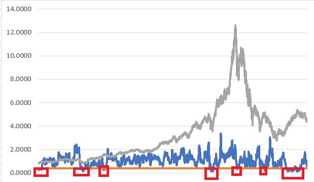
Figure 1 displays the growth of $1,000 invested in both of the above on a buy-and-hold basis from January 1980 through June 2019.Figure 1 – Growth of $1,000 invested in Small-Cap Value (blue) versus S&P 500 Index (orange); 12/31/1979-6/30/2019

Sure enough, the good news is that small-cap value has outperformed the S&P 500 Index by a factor of 1.48-to-1 (+11,486% versus +7,746%). The bad news is that the returns were quite volatile and cannot necessarily be described as “consistently better”.

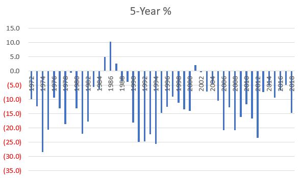
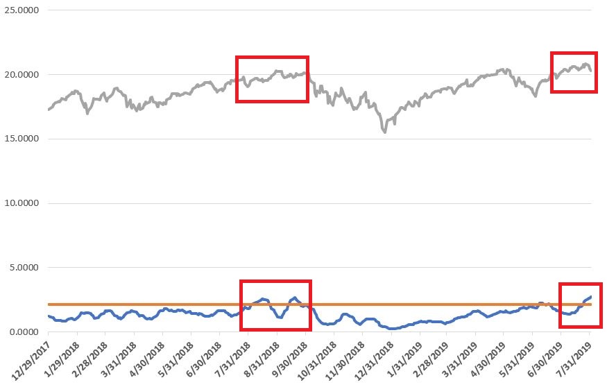
To illustrate, Figure 2 displays the growth of small-cap value divided by the growth of the S&P 500. When the line is rising it means small-cap value is outperforming and vice versa. As you can see there is a lot of give and take along the way. Small-cap value had a strong period of outperformance in the middle but before and after that the S&P 500 has spent as much time outperforming as underperforming.

From November 2016 through June 2019 the S&P 500 gained +38% versus only 11% for the S&P 600 Value Index. This type of underperformance makes it hard for investors to “sit tight” in small-cap value.Figure 2 – Ratio of Small-Cap Value to S&P 500

So, we will herein examine an approach that switches between the two indexes rather than just choosing one index or simply “splitting” money between the two.

The Test

At the end of each month we will measure the 12-month total return for both the S&P 600 Value Index and the S&P 500 Index.

If the 12-month total return for the S&P 600 Value Index is greater then we want to hold that index the following month, and vice versa.

One technical note: We are using total return data for our test (which includes price appreciation plus any dividend income). With the database that I use this data is not available until early in the next month so there is no way to do the month-end calculation and make a trade – if necessary – at the end of the month. For this reason, we will use a 1-month lag in applying trading signals as explained in the following example:

In say early January we get the December total return numbers for the two indexes. At that time, we will update the 12-month rate-of-change for each index as of the end of December. If the S&P 600 Value Index has a higher 12-month rate-of-change at the end of December, then at the end of January (the current month) we want to be long that index (i.e., as of the close of the last trading day of January). In early February we get the January total return numbers for the two indexes. At that time, we will update the 12-month rate-of-change for each index as of the end of January. If the S&P 600 Value Index has a higher 12-month rate-of-change at the end of January then we will simply continue to hold that index at least through the end of March. On the other hand, if at the end of January, the S&P 500 Index now has a higher 12-month rate-of-change then at the end of February we will sell the S&P 600 Value Index and buy the S&P 500 Index.

The Results

Starting 12/31/1979 through 6/30/2019:

*$1,000 invested in the S&P 600 Value Index using buy-and-hold grew to $115,862

*$1,000 invested in the S&P 500 Index using buy-and-hold grew to $78,460

*The average of these two is $97,161

*We will use a slightly modified approach as our benchmark. At the end of each calendar year we will rebalance so that both indexes start the new year with 50% of the portfolio. Using this approach, “splitting” money 50/50 each year between the two indexes grew to $102,839, or +10,184%

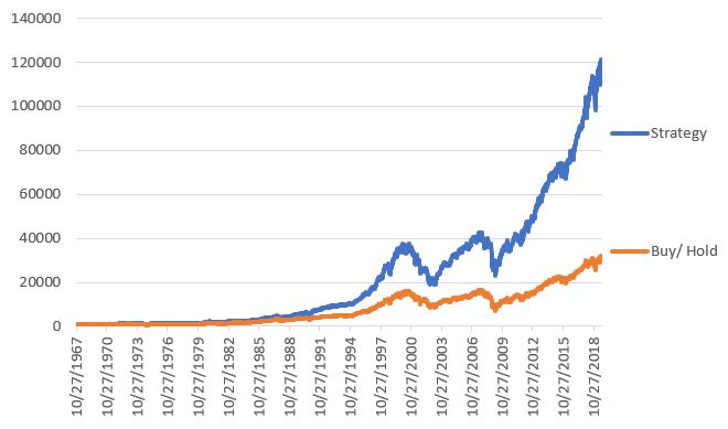
*During the same period, $1,000 invested using our switching method discussed above grew to $164,484, or +16,348%.

The results of the “Switching” versus “splitting” approaches appear in Figure 3.

Figure 3 – Growth of $1,000 invested using the “Switching” approach (blue) versus the “Splitting” approach (orange); 12/31/1979-6/30/2019

Review

It should be noted that the “Switch” method is by no means a “low risk”, or even a “lower risk” strategy. The maximum drawdown of -56.5% (during the 2008-2009 bear market) is a mindbender for most investors. Still, it is only slightly higher than buying and holding the S&P 600 Value Index (-53.3%) or the S&P 500 Index (-50.9%). And one can argue that an investor is well compensated for assuming any additional volatility or risk, as the “Switch” method gained +16,348% versus +7,746% for buying-and-holding the S&P 500 Index.

Figure 4 displays some comparative data.Figure 4 – Comparative Results

Other tidbits:

*The “Switch” approach outperformed the “Split” approach during 79% of all rolling 5-year periods

*In 473 months of testing, the “Switch” approach made 59 trades. This works out to an average of 1.5 trades per year. 13 years had 0 trades, 9 years had 1 trade, 6 years had 2 trades, 8 years had 3 trades and 3 years (1985, 1997, 2006) had 4 trades.

Summary

Is this any way to invest? That’s not for me to say. What we do know is that buying and holding small-cap value stocks has vastly outgained buying and holding the S&P 500 Index over the past roughly 39+ years (+11,486% versus +7,746%). Likewise, switching between small-cap value and the S&P 500 as detailed herein has performed buying and holding the S&P 500 Index by an even bigger amount (+16,348% versus + 7,746%).

Food for thought.

Jay Kaeppel