IMPORTANT NOTE: PLEASE READ THIS FIRST!  

I was alerted (by alert reader Satish) that the data that I have for ticker ULPIX is incorrect!

There is Bad News and Good News

The Bad News is that – and yes, this is embarrassing but – an alert reader noticed that the data that I have for ticker ULPIX is incorrect on several dates and as a result the performance numbers in the article below are incorrect.

The Good News is that there is still “a Happy Ending” in Part 3 which appears here.  So while you can read the article below for the calculations that will ultimately be used in Part 3, remember that the performance numbers are incorrect.

For the record, here is what happened: Under the category of “from sources believed to be reliable” I have not reviewed the data that I have for ticker ULPIX in some time.  Which is a shame because as it turns out the data that I have for ticker ULPIX and appears to contain random dates with incorrect prices.  This ended up having the effect of mathematically improving performance, but did not reflect reality.  Instead of using SPY data in my initial test, I went straight to the ULPIX data.  Had I tested the results initially using SPY data instead of ULPIX data I would have noticed the discrepancy when I then went to use ULPIX data.

So two takeaways:

1) Yes, this is embarrassing and I should have verified that the data I was using was accurate before “going to press”.  So I apologize for that.

2) Don’t give up on this whole “Trading Stocks using Bonds” thing until you read Part 3.

Jay Kaeppel

IMPORTANT NOTE: PLEASE READ THIS FIRST!  

I was alerted (by alert reader Satish) that the data that I have for ticker ULPIX is incorrect!

There is Bad News and Good News

The Bad News is that – and yes, this is embarrassing but – an alert reader noticed that the data that I have for ticker ULPIX is incorrect on several dates and as a result the performance numbers in the article below are incorrect.

The Good News is that there is still “a Happy Ending” in Part 3 which appears here.  So while you can read the article below for the calculations that will ultimately be used in Part 3, remember that the performance numbers are incorrect.

For the record, here is what happened: Under the category of “from sources believed to be reliable” I have not reviewed the data that I have for ticker ULPIX in some time.  Which is a shame because as it turns out the data that I have for ticker ULPIX and appears to contain random dates with incorrect prices.  This ended up having the effect of mathematically improving performance, but did not reflect reality.  Instead of using SPY data in my initial test, I went straight to the ULPIX data.  Had I tested the results initially using SPY data instead of ULPIX data I would have noticed the discrepancy when I then went to use ULPIX data.

So two takeaways:

1) Yes, this is embarrassing and I should have verified that the data I was using was accurate before “going to press”.  So I apologize for that.

2) Don’t give up on this whole “Trading Stocks using Bonds” thing until you read Part 3.

Jay Kaeppel

I have a pretty hard and fast rule about not being critical of other analyst’s work.  The reality of the markets is that no one ever really knows for sure what will happen next.  Sure some people get it right a lot more often than others (hence the reason some people get filthy rich in the markets and others do not).  But at any given point in time, two people can disagree on the outlook for a given stock, sector, commodity, etc. and only time will tell who is right.

See also An Example Commodity Play in SLV

OK, with all of that as a preface I saw an article recently titled (something like) “Is Now the Time for Housing Stocks?”  Truth be told I only read a small portion of the article but I think the gist of it was to suggest that now is a good time to buy housing stocks.  And if so, the author may ultimately prove to be correct.  But from my own analysis, I think I would have to answer the question posed in that article’s title as follows:

“Maybe, but Probably Not”

OK, granted that doesn’t exactly qualify as a “gutsy” call.  But historically the summer into fall months have not been kind to stocks in general and especially not to housing stocks.

Housing Stocks by Month

For our purposes we will us ticker FSHOX (Fidelity Select Construction & Housing Portfolio) as our proxy for housing stocks.  Figure 1 displays the percentage gain or loss achieved by FSHOX by month starting on 9/30/1988.Figure 1 – % Gained or Lost by month (ticker FSHOX; 9/88 to present)

As you can see in Figure 1, June and September have seen net losses of roughly -35% and -34% respectively.  July showed a modest net gain and August was basically a wash but with a small loss.  The rest of the months showed a net gain.

So let’s sum it up this way:

*June through September = (-53.1%)

*October through May = +2,336%

Figures 2 and 3 display the growth of equity during these two distinct bullish and bearish periods.Figure 2 – Growth of $1,000 holding FSHOX October through May (9/88-present)Figure 3 – Growth of $1,000 holding FSHOX June through September (9/88-present)

Clearly it is not as though housing stocks always rise between October and May, nor do they always decline between June and September.  Likewise, the “bullish” period clearly suffered a significant drawdown in the 2006-2008 period.  Still, even with that the net result was far superior to the “bearish” period results as displayed in Figure 3.

to put is as succinctly as possible,  a gain of +2,336% versus a loss of -53.1% is what we “quantitative types” refer to as “statistically significant.”

Figure 4 displays the annual gain/loss for the “bullish” months versus the “bearish” months.

Figure 4 – Annual Results for FSHOX (bullish periods versus bearish periods)

A few things to note appear in Figure 5:

Figure 5 – Comparative Results – Bullish Periods versus Bearish Periods for Housing stocks

Summary

It is important to note that none of the data presented in this article precludes the possibility that housing stocks will advance between now and the end of October this year.  Still if the question posed is “is now the time to buy housing stocks”, history suggests that the proper answer is:

“Maybe, but Probably Not”

So as a “Rule of Thumb”:

*Buy a house in the summer?  OK

*Sell a house in the summer?  OK

*Buy housing stocks in the summer?  Maybe not so much

Jay Kaeppel

Please note the use of the word “Example” in this article’s title.  Note also the lack of the word “Recommendation” and note especially the lack of words such as “You”, “Can’t” and “Lose”.

In my last article I noted that much of the commodity world seems to be at a fairly critical juncture.  After years of declines many commodities have been moving sideways to slightly higher and a number have touched multi-year support levels.  One such commodity is silver.  Now the truth is that I personally cannot make much of a bullish or bearish argument regarding where silver might be headed next.  But I do see some indications that it may be “moving” in a meaningful way soon.  So let’s look at why I say that and one example play on ticker SLV, the ETF that tracks the price of silver.

See also: A “Creative Play” in Natural Gas

Conflicting Elliott Waves

In Figure 1 we see that the weekly Elliott Wave count (as calculated by ProfitSource by HUBB) is pointing to the potential for lower prices in the months ahead.Figure 1 – SLV with Weekly Elliott Wave count (Courtesy: ProfitSource by HUBB)

On the other hand, in Figure 2 we see that the daily Elliott Wave count is pointing to the potential for higher prices in the weeks ahead.Figure 2 – SLV with Daily Elliott Wave count (Courtesy: ProfitSource by HUBB)

So which count is right – daily or weekly?  Unfortunately I have to go with my standard answer of “it beats the heck out of me.”  Still – adn interestingly – this does not preclude a trader from entering a position that can make money regardless of which Elliott Wave count proves to be correct (but which, alas, can lose money if neither wave count proves to be correct and silver remains in a trading range).

Example Trade

So to take it from “Soup to Nuts” so to speak, let’s assume that a trader:

*Has a $20,000 trading account

*Is willing to commit 5% to a single trade

*Would prefer not to risk the entire 5%

*Isn’t sure which way silver might move but is reasonably confident that SLV will break out of its recent trading range sometime in the not too distant future.

This sounds like a potential scenario for entering a long straddle using options, using no more than $1,000 ($20,000 x 5%).  Figure 3 displays the particulars for buying:

*8 August SLV 15.5 Calls @ $0.61

*8 August SLV 15.5 Puts @ $0.63

Figure 3 – Long SLV August 15.5 straddle (Courtesy www.OptionsAnalysis.com)

Figure 4 displays the risk curves for this trade, with each line representing the expected profit or loss based on the price for SLV as of a given date.  The distance between the black line and the green line at a price of $15.50 highlights the negative effect of option price time decay as option expiration draws near (i.e, if SLV is unchanged in price as expiration draws near both the call and the put will lose time premium at an accelerating rate which would increase the loss on the trade).

We can use this knowledge to help us plan how to manage this trade.Figure 4 – Risk curve for SLV straddle held to expiration (Courtesy www.OptionsAnalysis.com)

What we see in Figure 4 is the following:

*If this trade is held until expiration on 8/21 and SLV closes that day at $15.50 both options will expire worthless and the trade will lose $992.

*If SLV is between $14.26 and $16.74 on 8/21 this trade will show a loss.

*If SLV is above $16.74 or below $14.26 on 8/21 this trade will show a profit.

However, we do not have to hold this position until expiration if the opportunity arises to take an early profit.

Planning Trade Management

To zero in on “where this trade lives” let’s do the following:

*We will set the upper and lower price targets to the upper and lower Elliott Wave price targets that appear in Figures 2 and 1 respectively – in other words, an upper target of $17.31 and a lower target of $13.26.

*We will plan on exiting the trade no later than 8/7, which is 14 days prior to August expiration.  This will limit the potential damage due to time decay.

This plan gives us the scenarios that appear in Figures 5 and 6.Figure 5 – SLV Straddle held through 2 weeks prior to expiration (Courtesy www.OptionsAnalysis.com)Figure 6 – Risk curves for SLV straddle through 2 weeks prior to expiration(Courtesy www.OptionsAnalysis.com)

*In Figure 5 we see that although we still have to put up the full $992 to enter the trade, if we exit by 8/7 the likely “worst case” scenario is a loss of roughly -$538.  The bottom line is that if SLV remains inits recent trading range then this trade will lose money.

In Figure 6 we see that:

*If price hits the upper target of $17.31 then the profit will range from roughly $490 to $600, depending on how soon that price is hit.

*If price hits the lower target of $13.26 then the profit will be in the $750 range.

Summary

I cannot state that this will turn out to be a good trade. It sure is a pretty example though of one way to play a market that:

*Has been consolidating and/or bouncing off of support

*Has some expectation of making a move in some direction (based on daily and weekly Elliott Wave counts in this example)

*Offers a decent tradeoff between reward and risk if traded using options.

There may be more opportunities shaping up within the “exciting world of commodities.”  With many commodities markets at critical junctures now seems like a good time to start exploring other similar opportunities.

Jay Kaeppel

See also A “Creative Play” in Natural Gas

Commodity prices overall have taken a significant tumble over the past several years.  At the moment a number of commodity markets appear to be at least attempting to “form a bottom.”

I should probably point out up front that there is no “prediction” built into the comments above.  I don’t really have a firm opinion as to whether commodity prices are in the process of “bottoming out”, or if another round of “breakdowns” are in the offing.  The one thing I do sense is that there is a lot “hanging in the balance” in the near future.  To wit, please see Figure 1.

The charts in Figure 1 display:

DBA – which tracks agricultural commodities

DBC – which tracks an index of commodities

DBP – which tracks precious metals

JO – which tracks the price of coffee (also referred to by my wife as the “World’s Most Important Commodity”)

(click to enlarge)Figure 1 – Which way for Commodities?; tickers DBA, DBC, DBP, JO (Courtesy: ProfitSource by HUBB)

As you can see in Figure 1, all four of these commodity related ETFs have:

A) Declined significantly in recent year

B) Are attempting to form a bottom

As I mentioned I can’t really offer a meaningful opinion here as to “which way next”.  The one thing I do know is that traders looking for opportunities should be watching to see if these (and other commodity related assets) “bottom out” or “break down” again.  For now we need to sit and wait and see how this plays out.

For those of us who like “action”, we must currently heed the immortal words of that great philosopher Tom Petty, “the waiting is the hardest part.”

Jay Kaeppel

In a recent article I highlighted the fact that natural gas has showed a tendency to advance during a particular 3-day period in June.  Well, thanks to a strong rally on Day 3 this trend technically rang up another “success” in 2015.  But in reality, it was basically a wash to a small loss, depending on how one chose to play.

*July Natural gas futures declined $20 in value from 2.891 to 2.889.

*Ticker UNG advanced (such as it is) from $14.02 to $14.03.

*The June UNG 13 strike price call – if bought and sold at the market – was bought at $1.10 and sold at $1.07, or a $3 loss per contract.

Now onto the “Seasonally Unfavorable” period.

Jay Kaeppel

Well I hate to repeat myself, but the close of trading on 6/15 signals the start of one of the most consistently bearish seasonal periods in any market.  It marks the beginning of a bearish seasonal period for natural gas which extends through the end of July Trading Day #14 (July 21st in this case).

Figure 1 displays the net performance that a trader would have “achieved” by holding a long position in natural gas futures during this period every year since natural gas futures started trading in 1990 (and let be honest, “achieved” may not be exactly the best choice of words).Figure 1 – Long natural gas futures during bearish June/July period (1990-2014)

To note:

*Natural gas lost ground 19 years in a row from 1993 through 2011.

*Natural gas has lost ground in 21 out of the last 22 years during this period

*The one time it showed a significant gain was during the only previous year in which I actually mentioned this trend, 2012 (proving once again that Murphy’s Law is alive and well).

So forget all that, the real question is “what happens this time around?”  I can tell you that I have spent (wasted?) a significant amount of time trying to come up with a good “confirming” indicator to help suggest whether the trend will play out as expected during a given year but to no avail.  So let’s just consider the trading possibilities.

The Possibilities

So either you put some faith in the fact that natural gas has been down 21 out of 22 years during this period, or you don’t.  All of this leads to a variety of possibilities:

*Do Nothing: If you think seasonal trends are not to be trusted then by all means you should simply steer clear.  No harm, no foul.

*Short Natural Gas Futures: If you are well capitalized, willing to accept a certain degree of risk (and are not terribly frightened regarding what happened the last time I mentioned this trend, i.e., a sharp rally for natural gas rather than a decline), then the “purest play” is to sell short natural gas futures.  But make no mistake, selling short any futures contract involves an above average degree of risk.  As I write, July NG futures are trading at roughly $2.800.  With NG futures a $0.001 move in price is worth $10.  So if a trader sold short a futures contract at $2.800 and NG happened to advance to $3.000, the trader would lose $2,000.  So clearly selling short futures contracts is not for the faint of heart nor the under capitalized.Figure 2 – September Natural Gas Futures (Courtesy: ProfitSource by HUBB)

*Sell Short Shares of UNG: Another choice for non-futures traders is to sell short shares of ticker UNG, the ETF that (ostensibly) tracks the price of natural gas.  Selling short shares of any ETF is also generally considered to be a “risky” strategy.  There are margin requirements for maintaining the position not to mention that pesky little “unlimited risk” thing associated with selling short.  Still, for a trader willing to assume the risks, selling short shares of UNG is a “direct play” on lower natural gas prices.Figure 3 – ETF ticker UNG  (Courtesy: ProfitSource by HUBB)

*Buy an Inverse ETF: Ticker DGAZ is a triple-leveraged inverse ETF that tracks natural gas and trades roughly 9 million shares a day.  This sounds like a great choice for playing the bearish side of natural gas, but one needs to consider the potential “bad” along worth the potential “good.”  During the June/July “bearish” period in 2014 DGAZ gained +74.9%.  However, during the June/July bearish period in 2012 DGAZ lost -53.6%.  So if things “go wrong” with a triple-leveraged inverse ETF, things go “very wrong.”Figure 4 – ETF ticker DGAZ  (Courtesy: ProfitSource by HUBB)

*Put puts on UNG: This seems like a natural choice to play a potentially bearish trend.  The problem is that UNG options often have relatively wide bid/ask spreads.  For example, as I write the July Week 4 14 strike price put trades at $0.66 bid/$0.79 ask.  The bottom line is that if you buy a UNG put option and UNG only declines a few percent the trade will probably not make money.

*Use Options “Creatively”:  I mentioned in a recent article that traders often need to “get creative” in order to make money during the summer months, so let’s look at one “creative way” to play the short side of natural gas (without the risk associated with selling short futures or ETF shares).

The trade we will consider involves:

*Buying 3 October UNG 13 strike price puts

*Selling 2 July UNG 13 strike price puts

Note: For illustrative purposes we will use a “market order” (i.e., buying at the ask price and selling at the bid price).  Because of the width of the bid/ask spreads traders may consider using a limit order instead.  But for our purposes we are essentially assuming a “worst case” fill.

Figure 6 displays the particulars of the trade and Figure 7 displays the risk curves.Figure 6 – UNG Oct/Jul Directional Bear Put Spread (Courtesy www.OptionsAnalysis.com)

Figure 7 – UNG Oct/Jul Directional Bear Put Spread (Courtesy www.OptionsAnalysis.com)

Important things to note:

*The key factor in this trade is that fact that the July options will expire on 7/17, i.e., near the end of the bearish period (July 21^st).  This allows time decay to work for us as the July options will lose time premium at an accelerating rate as expiration nears.

*The October puts will not lose time premium as quickly. Note in Figure 2 that the July 13 put shows a Theta of -$0.90 – meaning it will lose roughly $0.90 a day due to time decay; the October 13 put shows a Theta of only -$0.50.  This explains the “bulge” in the purple risk curve line in Figure 3.  As July expiration draws near, accelerated time decay increases the profit potential.

*By buying in 3×2 ratio we retain unlimited profit potential in the event that natural gas does in fact decline sharply.

*If Murphy decides to invoke his dreaded Law and whack me upside the head again for daring to mention this bearish seasonal trend in natural gas again, the most that this trade can lose by July 21^st is $220 (and that is only if UNG rallies roughly 50%; if UNG rises roughly one standard deviation to around $16 a share, the loss on this trade is roughly -$150.

Summary

As always, none of this constitutes a “recommendation”, only “possibilities”.  In any event, a trader first must decide if they really want to risk their hard-earned money on a seasonal trend.  Then they must decide how they want to go about making the play.  As you have seen there are “high risk/high reward” possibilities, and there are other not high risk/high reward ideas.

In most cases I prefer taking a limited risk using a reasonable amount of trading capital and hoping for a high percentage rate of return on the capital invested.  What you may choose to do is of course entirely up to you.

But whatever you decide to do, DO NOT breathe a word of this to Murphy…

Jay Kaeppel

See also Jay Kaeppel Named Portfolio Manager for New Investment Program

Note the use of the word “play” in the title, and the lack of the word “recommendation.”  I recently wrote here about the fact that natural gas has showed a historical tendency to advance over the three days encompassed by June trading days number 9, 10 and 11.  This is clearly a speculative idea and granted, one that the majority of traders are not inclined to “jump on.”

But for illustrative purposes, when it comes to playing purely speculative ideas there are usually a variety of ways to play.  To wit, a trader could make one of the following trades at the close:

1) Enter a long position at the close in natural gas futures and hold for three days;

2) Buy 100 shares of ETF ticker UNG, trading at $14 as I write, or $1,400.

3) Buy 1 June UNG 13 strike price call (as I write trading at $1.02 bid/$1.10 ask – i.e, if bought at the market would cost $110).

So if things were unchanged by the close of trading a trader could enter a call option position for a total cost (and risk) of $110 by buying the June UNG call option.

Summary          

The purpose here is not to try to prompt you to enter a trade in natural gas.  I basically just want to follow through with keeping up to date on an idea I wrote about a little while ago and to alert you to the fact that there are “low risk” ways to let the “wild-eyed speculator” in you out of its cage once in a while – i.e., in this case via a cheap, in-the-money call option.

Jay Kaeppel

See also Jay Kaeppel Named Portfolio Manager for New Investment Program

Keep a close eye on crude oil.  As I write crude is breaking out above a declining upper trend line as seen in Figure 1.  Whether this breakout proves to be “for real” or a “fake out” may well have important implications moving forward.

Figure 1 – Crude Oil attempting to breakout to the upside (Chart courtesy of www.Barchart.com)

As you can see in Figures 2 and 3 (and as I wrote about here), both the daily and weekly Elliott Wave counts for crude are pointing decidedly to the bearish side. Figure 2 – Daily crude oil with Elliott Wave count (Courtesy: ProfitSource by HUBB)

Figure 3 – Weekly crude oil with Elliott Wave count (Courtesy: ProfitSource by HUBB)

Look for one of two scenarios to develop from here:

1) The current breakout proves to be “for real” and the bearish Elliott Wave counts go “poof” and vanish into the ether (and don’t you just hate that about Elliott Wave counts?)

2)The current breakout proves to be a “fake out” and crude reverses back to the downside.

If crude does reverse back to the downside after this current pop runs its course, then the likelihood of another serious leg down for crude increases greatly.

Now this is what I call a potential “Summer Blockbuster” so I will be watching intently.  Hmm, where’s my popcorn?

Jay Kaeppel

Please see also Jay Kaeppel named Portfolio Manager for New Investment Program

I last wrote about the fact that over the past 50 years, the Dow Jones Industrials Average has gained almost exactly zero net points during the months of June, July and August.  I also highlighted the fact that in light of this performance, investors and traders might need to get a little “creative” if they actually wish to make money during these months.  So this time out, let’s “get a little creative” and highlight one possible way to potentially take advantage of “summer boredom.”

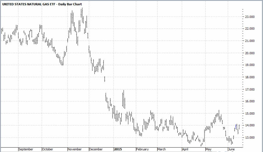
(For other “Summer Strategies” see Jay’s recent posts: Will Natural Gas Break Wind in June? and Will Natural Gas Soar With the Wind in June?

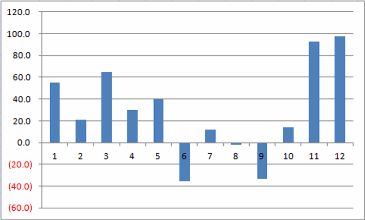
This method involves a simple, commonly used option trading strategy.  So of course, if you have no interest in options then you are free to stop reading here.  Thanks for checking in and please come back soon.  But before you sign off you might want to take one more glance at Figure 1 here and verify that you have no interest in considering alternatives to just “riding the market” for the next several months.  (If you are an option trader please see the Special Offer to JayOnTheMarkets.com readers here).

Jay’s How to “Enjoy Summer Boredom” (ESB) Strategy

This method is based on the theory that big stock market moves in the summertime have shown a historical tendency to (WARNING: Impending “Highly Technical Trading Term”) “peter out”.  However, this does not mean that every time a stock shoots higher for a few days that it marks a major top and signals an impending sharp decline.  It is just not an uncommon event for a given stock to pop higher and then “meander” sideways to lower for a period of time.  One way to potentially take advantage of this situation with stocks that you do not hold is to enter into a bear call credit spread.  This involves selling an at-the-money or out-of-the-money call option on a stock or index and simultaneously buying a further out-of-the-money call option on the same stock or index.  More money is taken in for the option sold than is paid out for the option bought.

Hopefully as the stock “meanders” sideways to lower, the options lose value and the position can eventually be bought back (or expire) for less than the amount received when the position was entered.  The example that follows should answer any questions about the mechanics of the bear call credit spread.

Jay’s ESB Trading Rules:

-Today is during the months of June, July or August

-The 2-day RSI for a given stock or index is >=90

-The 14-day ADX value for that stock is below 25

-Ideally at least 1,000 options are traded per day for the stock in question and the bid/ask spreads are 2% or less

(A higher degree of confidence if ticker SPY or QQQ or RUT or VTI also show a 2-day RSI>=80 and/or if the 2-day RSI rises to 80 or above and then reverses for one day; but this is not a requirement)

-When this setup occurs selling an at-the-money or out of the money call option with 14 to 45 days left until expiration and buying another higher strike price call option.

Example

As you see in Figure 1, on 7/15/14 the 2-day RSI for SPY reversed lower after topping 80%.Figure 1 – SPY 2-day RSI reverses lower from above 80% (Courtesy: www.AIQSystems.com)

From here all of the analysis is done using www.OptionsAnalysis.com the software I use for all of my, well, option analysis, what else?  (If you are an option trader please see the Special Offer to JayOnTheMarkets.com readers here).

We first go to Web Site | Lists | Filter List. The settings in Figure 2 are used to find stocks that have reasonable option volume and reasonably tight bid/ask spread on those options.

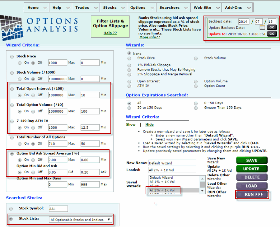
(Click on Figures below to enlarge them)Figure 2 – Looking for good option volume and tight bid/ask spreads (Courtesy www.OptionsAnalysis.com)

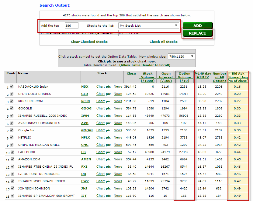
As you can see in Figure 3, this leaves us with 386 “high option volume, tight bid/ask spread” candidates.Figure 3 – Stock List Filter Output; 386 high option volume, low bid-ask spread candidates  (Courtesy www.OptionsAnalysis.com)

We save these stocks to a “My Stock List” then go to Stocks | Rankers | RSI.

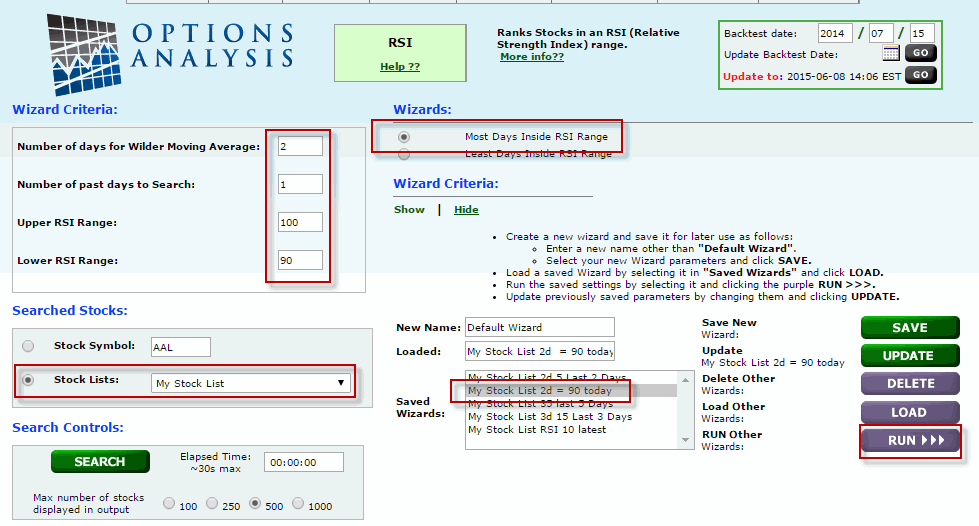
Figure 4 displays the input screen which allows us to look through the 386 tocks we just saved and find only those that have a 2-day RSI reading of 90% or higher.Figure 4 – Finding Stocks with 2-day RSI >= 90 (Courtesy www.OptionsAnalysis.com)

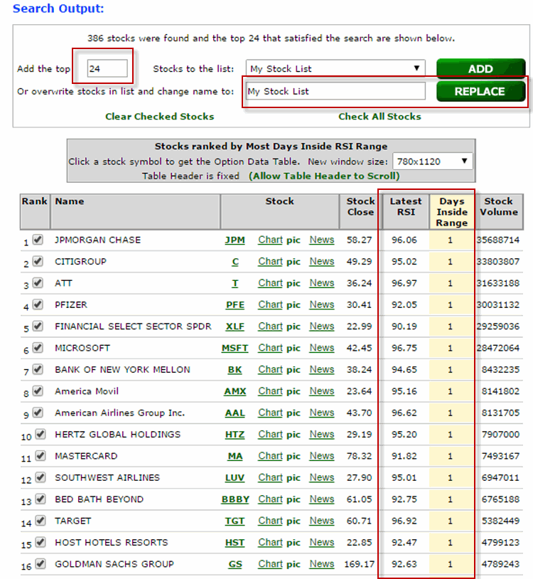
Figure 5 displays the output.  We now have 24 stocks that meet our option volume and option bid-ask spread requirements and 2-day RSI readings >=90%. We save these by overwriting My Stock List with these 24 securities by clicking “Replace”.Figure 5  – Stocks with 2-day RSI >= 90 (Courtesy www.OptionsAnalysis.com)

*Next we go to Searchers | Multi-Strategies | Find Trades II.

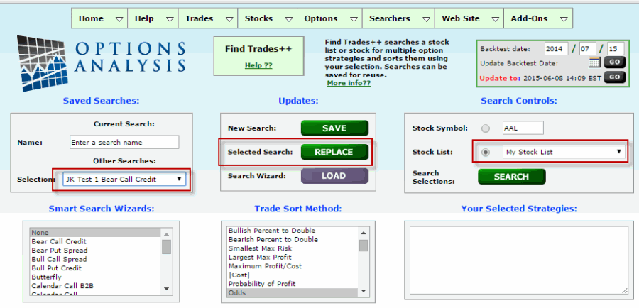
In this routine I have created a “Wizard” for finding bear call credit spreads.  This Wizard is selected by selecting “JK Test 1 Bear Call Credit” under “Saved Searches” and clicking “Replace” as shown in Figure 6.Figure 6 – Selecting Jay’s Bear Call Credit Spread Saved Search (Courtesy www.OptionsAnalysis.com)

This selects the bear call credit spread strategy and sets the default strategy inputs displayed in Figure 7.

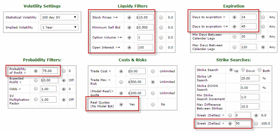
Figure 7 – Jay’s Bear Call Credit Input Criteria Settings (Courtesy www.OptionsAnalysis.com)

Among these inputs are:

*A Probability of Profit of 75% or more

*Stock Price >= $10

*Minimum sell price for an option is $0.50

*Minimum Option Volume is 1

*Minimum Option Open Interest is 100

*An option must have an active “Real Quote” in order to be considered

*Between 14 and 45 days left until expiration

*The call option sold must have a Delta of less than50.

Not shown is the fact that the selected “Sorting Criteria” is “Expected Profit/Risk.”

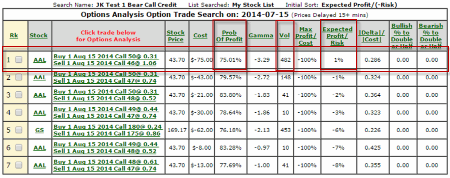
Figure 8 displays the trade output screen. In this case all of the top suggested trades were for ticker AAL.Figure 8 – Multi-Strategies Output screen (Courtesy www.OptionsAnalysis.com)

If we click on the top trade we get the particulars for that trade which appears in Figure 8.  Note that I arbitrarily chose to display this trade as a 10-lot.  This trade involves:

*Selling 10 AAL August 46 calls

*Buying 10 AAL August 50 calls

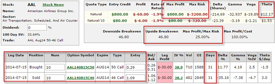
Figure 9 – AAL August 46-50 Bear Call Credit particulars (Courtesy www.OptionsAnalysis.com)

Key things to note about this trade:

*Maximum profit potential = $800

*Maximum risk = $3,200

*Current stock price = $43.70

*Breakeven price = $46.80

*31 days left until option expiration

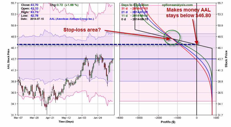
Figure 10 displays the risk curves for this trade.  Each of the four colored lines displayed represents the expected $ profit or loss at a given stock price for four different dates.  Below the breakeven price of $46.80 we see the lines drifting to the right (further into the profit zone).  This illustrates the potentially positive effect of time decay working in our favor.Figure 10 – Risk curves for AAL August Bear Call Credit Spread (Courtesy www.OptionsAnalysis.com)

So Then What?

So let’s assume this trade was entered just as displayed in Figures 9 and 10. A trader has to decide (actually for the record these decisions should be made before entering the trade) when to take a profit and when to cut a loss.  As with many things in trading there are no “Perfect Rules”.  And in fact, there are too many possibilities to lit and discuss here.  So let’s just choose some for examples sake and see what happened going forward.

Profit Taking Ideas:

*If the 3-day RSI drops below 25% and we have a profit of any amount we may consider closing half of the open position.

*If we achieve an open profit of 20% or more prior to expiration (remember 25%, i.e., $800 / $3,200 – is our maximum profit potential) we may consider taking a profit and closing the entire position.

*As long as stock remains below price of option sold ($46) we can consider holding the position until option expiration.

Loss Cutting Ideas:

*If the stock breaks out above recent resistance at $44.88.

*If the position shows an open loss above $x (each trader needs to decide for themselves what value x should be)

*Cut a loss in the area where the various risk curve lines cross – in this case that is somewhere between $46.80 and $47.50.  Again, each trader would need to decide for themselves.

So for example purposes, we will:

*Exit with a loss if AAL reaches or exceeds $46.80.

*Exit with a profit of 20% or more.

 The Result

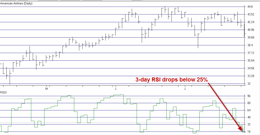
As you can see in Figure 11, by 7/28 AAL stock had fallen to $40.29 a shares, the 3-day RSI had dropped below 25%.Figure 11 – AAL stock declines triggering a profit-taking opportunity

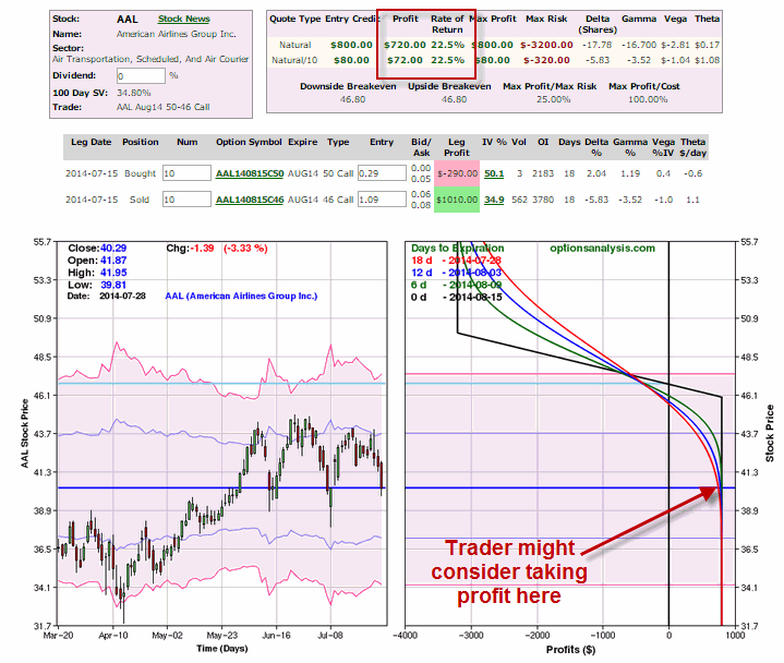
As you can see in Figure 12, at this point the trade was showing an open profit of $720 or 22.5%.  At this point a trader could have closed the trade generating a profit of 22.5% in 13 calendar days.Figure 12 – AAL Bear Call Credit profit-taking opportunity (Courtesy www.OptionsAnalysis.com)

Summary

Now comes the important part.  Repeat after me: “Not every trade will work out as well as this one.”  Please repeat that phrase two or three, um, hundred times before proceeding.

The trade in this example serves only as an illustration.  The key thing to note is the process which is intended to find trades that can put the odds in your favor and potentially take advantage of the “summer doldrums”.

Jay Kaeppel