IMPORTANT NOTES:
In case you missed my updates to Part 1 and Part 2: the data that I had for ticker ULPIX (which is a ProFunds mutual fund that tracks the S&P 500 Index times 2) contained bad days of data, which as it turned out, overstated the returns that I showed in the articles.
That’s the Bad News. The Good News is that the goal of the articles was to ultimately demonstrate that “combining” two different methods can oftentimes prove very worthwhile. As it turns out, that is the case here – granted, not as dramatically so as I had originally thought, but, well see for yourself………
In Part 1 and Part 2 I detailed two separate methods for trading a stock index mutual fund (or ETF) using the relationship between the S&P 500 Index and junk bonds as the catalyst.
The natural question that might pop into most people’s head is “so which one is best?” In this case, I think the proper response is “why choose?” For here’s the interesting thing when it comes to trading. Sometimes (though granted, not always) “combining” two systems can offer a better tradeoff between reward and risk than simply “choosing” one or the other. So in this article let’s take a look at what might have happened had a trader combined the methods I detailed in Parts 1 and 2.
The Premise
We will combine the “44-Day SPY/HYG Ratio System” (System 1 for short) and the “252-Day Rate-of-Change System” (System 2 for short) and measure the results.
The Particulars
*For our “stock” component we will use ticker SPY (the ETF that tracks the S&P 500 Index”
*For our junk bond component we will use ticker HYG (the iShares high yield corporate bond ETF, which started trading in April of 2007)
*Because we are shooting for maximum returns I originally used data ticker ULPIX (which is the leveraged ProFunds mutual fund that seeks to track the daily change for the S&P 500 Index times 2). Unfortunately, the data that I have for ULPIX contains errors on enough days to make a difference. So for performance purposes I will simply multiply the daily return for ticker SPY times 2 as a proxy for ULPIX.
*When we are out of ULPIX we will simply hold cash. For our purposes, an annual rate of 1% of interest is used.
We will start our test on 4/11/2008 (rather than 12/31/2007 for the test in Part 1) because HYG started trading on 4/11/2007 and we need 252 trading days to make our first 252-day rate-of-change calculation.
The Calculations
System 1: The 44-day Ratio Moving Average
A = SPY / HYG (each trading day)
B = 44-day simple moving average of A
C = (A – B)
If C > 0 then at the next close Buy (or continue to hold if already long) ticker ULPIX
If C< 0 then at the next close Sell ticker ULPIX and move to cash (or remain in cash if C was previously less than 0).
System 2: The 252-day Rate-of-Change
A = SPY today / SPY 252 trading days ago
B = HYG today / HYG 252 trading days ago
C = (A – B)
If C > 0 then at the next close Buy (or continue to hold if already long) ticker ULPIX
If C < 0 then at the next close Sell ticker ULPIX and move to cash (or remain in cash if C was previously less than 0.
Combined Model:
*If System 1 is”bullish” we will add +1 point to the Combined Model.
*If System 2 is “bullish” we will add +1 point to the Combined Model
*If the Combined Model reading is greater than 0 (i.e., if EITHER system is bullish) then at the next close Buy (or continue to hold if already long) ticker ULPIX.
*If the combined reading is equal to 0 (i.e., if NEITHER of the systems are bullish at the same time) then at the next close Sell ticker ULPIX and move to cash (or remain in cash if the combined reading was previously 0).
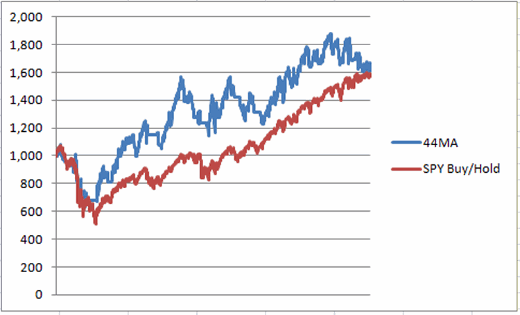
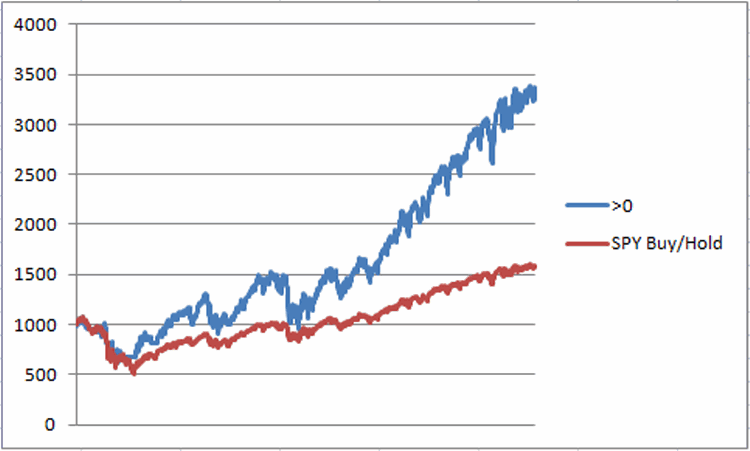
Figure 1 displays the growth of $1,000 achieved by holding SPY times 2 when System 1 is bullish and cash when it is bearish versus buying and holding SPY (no leverage). $1,000 using System 1 grew to $1,635 versus $1,581 for buying and holding SPY.
 Figure 1 – Growth of $1,000 using System 1 (blue) versus SPY (red); 4/11/2008-6/19/2015
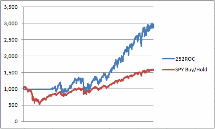
Figure 2 displays the growth of $1,000 achieved by holding SPY times 2 when System 2 is bullish and cash when it is bearish versus buying and holding SPY (no leverage). $1,000 using System 1 grew to $2,921 versus $1,581 for buying and holding SPY. Figure 2 – Growth of $1,000 using System 2 (blue) versus SPY (red); 4/11/2008-6/19/2015
Now let’s look at market performance when we combine the two systems.
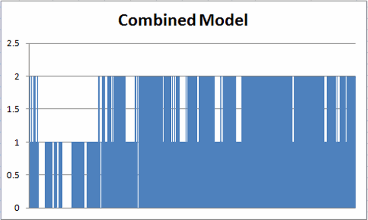
Figure 3 displays the daily combine reading for all days from 4/11/2008 through 6/19/2015.
 Figure 3 – Combined Model Readings; 4/11/2008 – 6/19/2015
When the blue line in Figure 1 is greater than 0 then the system is long ULPIX and when the blue line is at 0 the system is in cash.
The Results
*As you can see in Figure 3, throughout most of 2008 and much of 2009 the system was in cash. Since that time the Combined Model has been above 0 with one brief exception. Given that the stock market fell hard in 2008 and has mostly advanced steadily since this is about what you would hope to see.
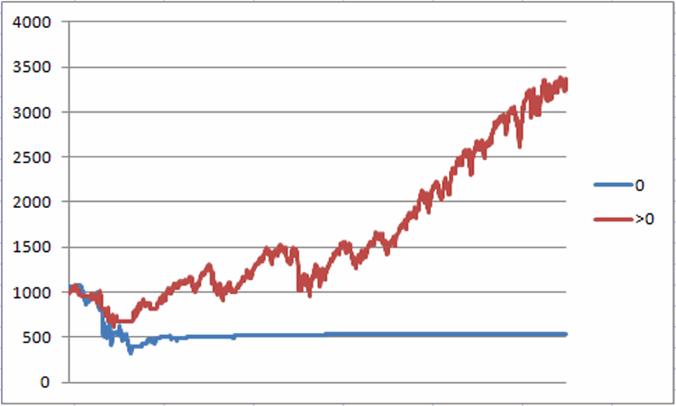
Figure 4 displays:
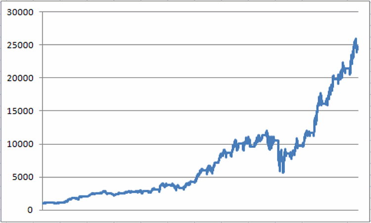
*The growth of $1,000 achieved by holding SPYx2 when the Combined Model reads +1 or +2 and holding cash when the combined model is 0 (red);
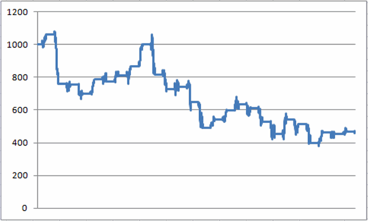
*The growth of $1,000 achieved by holding SPYx2 when the Combined Model reads) 0 (blue);
 Figure 4 – Growth of $1,000 holding SPYx2 when Combined Model > 0 (red line) versus growth of $1,000 holding SPYx2 when Combined Model = 0 (blue line); 4/11/2008 – 6/19/2105
Finally, Figure 5 displays:
*The growth of $1,000 achieved by holding SPYx2 when the Combined Model reads +1 or +2 and holding cash when the combined model is 0 (red);
*The growth of $1,000 achieved by holding SPY on a buy-and-hold basis
 Figure 5 – Growth of $1,000 holding SPYx2 when Combined Model > 0 (red line) versus growth of $1,000 buying and holding SPY (blue line); 4/11/2008 – 6/19/2105
In sum;
*A original $1,000 invested in SPYx2 when the Combined Model is > 0 and in cash when the Combined Model is 0 grew to $3,305, or +230%.
*A original $1,000 invested in SPYx2 when the Combined Model is = 0 and in cash when the Combined Model is > 0 declined to $566, or a loss of -43%.
*For comparison sake, $1,000 invested in ticker SPY on a buy-and-hold basis grew to $1,581, or +58.1% during the same time.
As I am wont to say, the difference between +230% and -43% is what we “quantitative analysis types” refer to as “statistically significant.”
Figure 3 displays the annual returns based on:
*Holding SPYx2 when the Combined Model > 0 versus
*Holding SPYx2 when the Combined Model is = 0 verus
*Buying and holding SPY (no leverage)
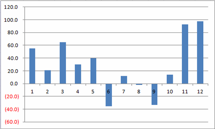
 Figure 6 – Annual Returns for Combined Model Readings of > 0 versus Combined Model readings of 0 and buying and holding SPY
*- Starting on 4/11/2008
** – through 6/19/2015
***Average annual return 2008 through 2014
Summary
So is this SPY/HYG Combined Model a “World Beater” system that everybody should adopt? Probably not. The test period is short (7+ years), the maximum drawdown was large (-42%) and much of the outperformance was based on using leverage and so on.
But the real purpose of this article is not to convince you to use this particular system. The real purpose is simply to illustrate how combining two methods (one that gained +64% and the other that gained +192% can improve the overall net result (+230%).
The fact that this method produced an annual return of +22.7% versus +8.3% for the S&P 500 suggests that there may (at times) be some truth to the notion that “two ideas are better than one”.
Jay Kaeppel
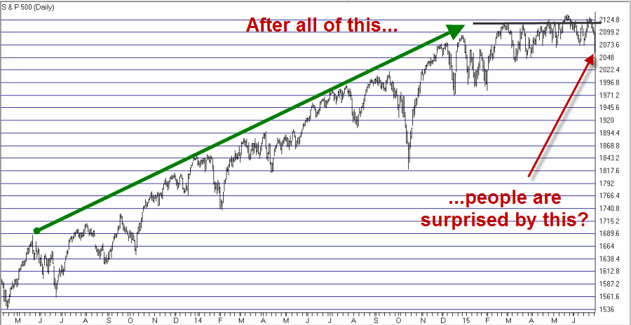 Figure 1 – Major long-term advance followed by an extended topping formation, followed by, well, what else?
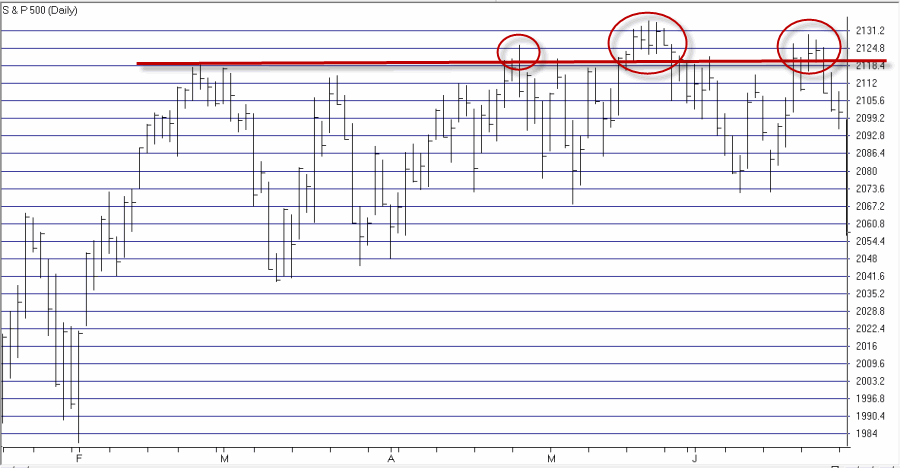 Figure 2 – When price tries time and again to breakout but cannot the market is (usually) telling you something important
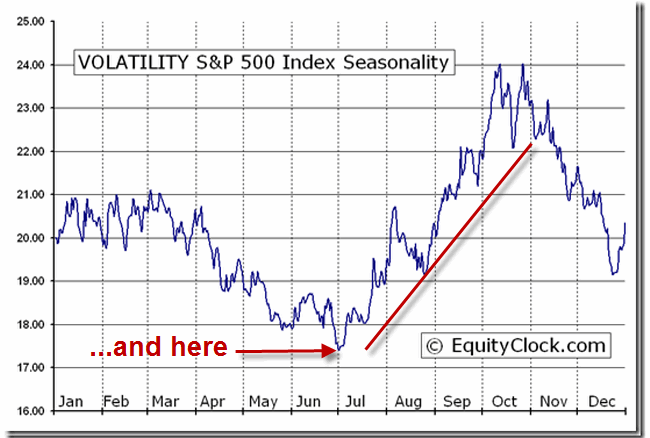 Figure 4 – Volatility “spikes” are not uncommon during the summer months (Courtesy: www.EquityClock.com)